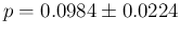
The pdf of  , given the set of conditions
  , to which we have
added
, to which we have
added  and
and  in order to remind that it also depends on the
chosen family for the prior, is finally
in order to remind that it also depends on the
chosen family for the prior, is finally
So, although we have not been able to get an analytic solution,
which for problems of this kind is out of hope,
we have got an expression for
 ,
that we can compute numerically and check against the JAGS results seen in Sec.
,
that we can compute numerically and check against the JAGS results seen in Sec. ![[*]](crossref.png) .
For the purpose of this work, we did not put particular effort
in trying to speed up the calculation
of Eqs. ()-() and therefore the comparison
concerns only the result, and not the computer time or other technical
issues. The agreement is excellent, even when we are dealing with
numbers as large as 10000 for
.
For the purpose of this work, we did not put particular effort
in trying to speed up the calculation
of Eqs. ()-() and therefore the comparison
concerns only the result, and not the computer time or other technical
issues. The agreement is excellent, even when we are dealing with
numbers as large as 10000 for  (and a few thousands for
  ).
For example, the comparison using
the same values of
).
For example, the comparison using
the same values of  and
and  of Sec. is shown in the upper plot of Fig. :
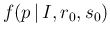
Figure:
Direct computation of Eq. () (solid lines)
vs JAGS results (histograms) for the flat prior
(magenta dashed line) and for a
Beta (magenta dotted line).
Upper plot: and . Lower plot:
(magenta dotted line).
Upper plot: and . Lower plot:  and
and  .
.
 |
- The histogram peaked around
 is the JAGS result obtained by
 iterations,
with over-imposed the pdf evaluated making use of Eq. (),
starting from a uniform prior (magenta dashed line).
In terms of expected value
iterations,
with over-imposed the pdf evaluated making use of Eq. (),
starting from a uniform prior (magenta dashed line).
In terms of expected value  standard uncertainty
the direct calculation (exact - see Eq. () and Appendix B.13) gives
standard uncertainty
the direct calculation (exact - see Eq. () and Appendix B.13) gives
 versus
 of JAGS
(with exaggerated number of decimal digits just for detailed comparison).
of JAGS
(with exaggerated number of decimal digits just for detailed comparison).
- Then we have changed the prior, choosing one strongly
preferring high values of (dotted magenta curve)
with rather small uncertainty:
a
Beta, yielding
an expected value of 0.60 with standard deviation of 0.05.
This new prior has the effect of `pulling' the
distribution of on the right side. The agreement
of the results obtained by the two methods is again excellent,
resulting in
 and
and
 (direct and JAGS, respectively).
Then we repeat the game with a sample ten times smaller, that
is , and assuming (lower plot in the same figure).
Again the agreement between direct calculation and MCMC sampling
is excellent.
It is worth noting that the possibility to write down an
expression for the pdf of interest for an inferential
problem with several nodes, after marginalization
over six variables, has to be considered a lucky case,
thanks also to the approximation of modeling
the sampling by a binomial rather than a hypergeometric
and to the use of conjugate priors. The purpose of this
section is then mainly didactic, being the valuation
of the pdf's of other variables (and of several variables all together)
and of their moments prohibitive.
It is then clear the superiority of estimates based
on MCMC methods, whose advent several decades ago has been a kind
of revolution, which have given a boost to Bayesian methods
for `serious' multidimensional applications, tasks before
not even imaginable.58
![$\displaystyle \frac{1}{N_f}\cdot \Large [ p^{r_0-1}\cdot (1-p)^{s_0-1}\Large ]\...
...{P_I}} \cdot \binom{n_s-n_I} {n_P-n_{P_I}} \cdot
\binom{n_s}{n_I} \cdot \right.$](img933.png)
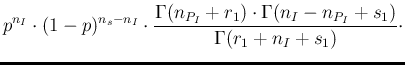
![$\displaystyle \left.\frac{\Gamma (n_P-n_{P_I}+r_2)\cdot \Gamma(n_s-n_I-n_P+n_{P_I}+s_2)}
{ \Gamma(n_s-n_I+s_2+r_2)} \right] \,.$](img903.png)