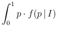
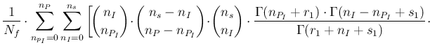
The normalization factor  is given by the integral
in d
is given by the integral
in d of this expression, once
  has been chosen.
As we have done in the previous section, we opt for
Beta
has been chosen.
As we have done in the previous section, we opt for
Beta ,
taking the advantage not only of the flexibility
of the probability distribution to model our `prior
judgment' on , but also of its mathematical
convenience. In fact, with this choice, the resulting term
in Eq. (
,
taking the advantage not only of the flexibility
of the probability distribution to model our `prior
judgment' on , but also of its mathematical
convenience. In fact, with this choice, the resulting term
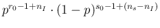
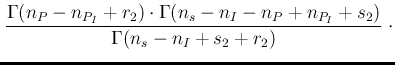
in Eq. (![[*]](crossref.png) ) depending on is given
by
) depending on is given
by
 . The integral
over from 0 to 1 yields again a Beta function, that is
B
. The integral
over from 0 to 1 yields again a Beta function, that is
B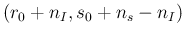 , thus
getting
, thus
getting
Similarly, we can evaluate
the expression of the expected values of and of  ,
from which the variance follows, being
,
from which the variance follows, being
 E
E E
E . For example,
being
E
. For example,
being
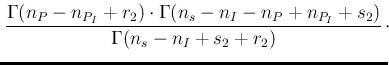
E given by
in the integral the term depending on
becomes
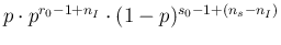 ,
increasing the power of by 1 and
thus yielding
,
increasing the power of by 1 and
thus yielding
while
E is obtained replacing `
 ' by
`
' by
`
 '. A script to evaluate expected value and standard deviation
of is provided in Appendix B.13.
'. A script to evaluate expected value and standard deviation
of is provided in Appendix B.13.
The expression can be extended to `
 ' by `
 ',
thus getting
E
',
thus getting
E and
E
and
E , from which
skewness and kurtosis can be evaluated.
Finally, making use of the so called
Pearson Distribution System implemented in R [14],
, from which
skewness and kurtosis can be evaluated.
Finally, making use of the so called
Pearson Distribution System implemented in R [14],
 can be obtained with a quite high degree of accuracy, unless
the distribution is squeezed towards 0 o 1, as
e.g. in Fig. .57 A script to evaluate mean, variance, skewness and kurtosis, and
from them by the Pearson Distribution System is shown
in Appendix B.14.
can be obtained with a quite high degree of accuracy, unless
the distribution is squeezed towards 0 o 1, as
e.g. in Fig. .57 A script to evaluate mean, variance, skewness and kurtosis, and
from them by the Pearson Distribution System is shown
in Appendix B.14.
 d
d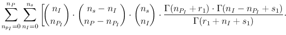
![$\displaystyle \left.\frac{\Gamma(r_0+n_I)\cdot\Gamma(s_0+n_s-n_I)}{\Gamma(r_0+s_0+n_s)}\right]$](img911.png)
![$\displaystyle \left.\frac{\Gamma(r_0+n_I\mbox{\boldmath$+1$})\cdot\Gamma(s_0+n_s-n_I)}
{\Gamma(r_0+s_0+n_s\mbox{\boldmath$+1$})}\right]\,,$](img924.png)