Updated knowledge of $\pi_1$ and $\pi_2$ in the case of `anomalous' number of positives

Let us imagine that, instead of 1150 positives, we `had observed' a much smaller number (in terms of standard deviation of prediction, that, we remind, is about 220). For example, an under-fluctuation of 3 $\sigma$'s would yield 490 positives. But let us exaggerate and take as few as 50 positives, corresponding to $-5\,\sigma$'s. The JAGS result (this time monitoring also $\pi_1$ and $\pi_2$), obtained using our usual uncertainties concerning $\pi_1$ and $\pi_2$ ( $0.978\pm 0.007$ and $0.115 \pm 0.022$, respectively), is showed in Fig. 

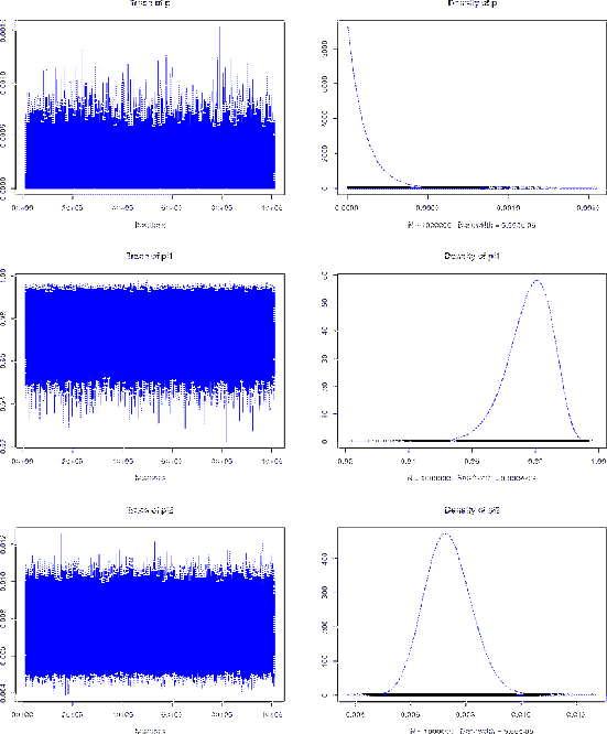
Figure: JAGS inference of $p$, $\pi_1$ and $\pi_2$ from $ns=10000$ and $n_P=50$ (see text).

and summarized as

1. Empirical mean and standard deviation for each variable,
   plus standard error of the mean:

         Mean        SD  Naive SE Time-series SE
p   0.0001022 0.0001023 1.023e-07      1.998e-07
pi1 0.9781819 0.0071445 7.145e-06      7.161e-06
pi2 0.0073581 0.0008463 8.463e-07      8.463e-07

2. Quantiles for each variable:

         2.5%       25%       50%       75%     97.5%
p   2.586e-06 2.949e-05 7.091e-05 0.0001415 0.0003771
pi1 9.622e-01 9.738e-01 9.789e-01 0.9833334 0.9899013
pi2 5.790e-03 6.771e-03 7.327e-03 0.0079113 0.0091035

As we see, the distribution of $p$ looks exponential, with mean and standard deviation practically identical and equal to $1.0\times 10^{-4}$ (we remind that it is a property of the exponential distribution to have expected value and standard deviation equal). In this case the quantiles produced by $R$ are particularly interesting, providing e.g. $P(p\le 3.77\times 10^{-4}) = 97.5\%$.

The fact that a small number of infectees squeezes the distribution of $p$ towards zero follows the expectations. More surprising, at first sight, is the fact that also the value of $\pi_2$ does change:

$$\pi_2: 0.115\pm 0.022 \ \ \longrightarrow \ \ 0.0074\pm 0.0008\,.$$

The reason why $\pi_2$ can change (also $\pi_1$ could, although JAGS `thinks' this is not the case) is due to the fact that it is now a unobserved node, and the Beta$(r_2,s_2)$ with which we model it is just the prior distribution we assign to it. In other words, the very small number of positives could be not only due to a very small value of $p$, but also to the possibility that $\pi_2$ is indeed substantially smaller than what we initially thought. This sounds absolutely reasonable, but telling exactly what the result will be can only be done using strictly the rules of probability theory, although with the help of MCMC, because in multivariate problems of this kind intuition can easily fail.⁵²