Quality of the inference as a function of the sample size and of the fraction of positives in sample

A more systematic study of the quality of the inference is shown in Tab. ,

Table: Proportion $p$ of infected in a population, inferred from the number $n_P$ of positives in a sample of $n_S$ individuals. The three blocks of the table corresponds to the assumptions summarized by $\pi_1=0.978\pm 0.007$ and $\pi_2 =(0.115\pm 0.022$, $0.115\pm 0.007$, $0.022\pm 0.007)$.

$n_s$	$[n_P]$
	E$(p)\pm \sigma(p)$
300	[34]	[60]	[86]	[112]	[138]	[164]
	$0.026\pm 0.019$	$0.100\pm 0.034$	$0.200\pm 0.036$	$0.299\pm 0.037$	$0.399\pm 0.037$	$0.495\pm 0.036$
1000	[115]	[201]	[288]	[374]	[460]	[546]
	$0.021\pm 0.015$	$0.099\pm 0.028$	$0.198\pm 0.026$	$0.298\pm 0.025$	$0.399\pm 0.024$	$0.498\pm 0.023$
3000	[345]	[604]	[863]	[1122]	[1381]	[1640]
	$0.018\pm 0.014$	$0.099\pm 0.024$	$0.198\pm 0.023$	$0.299\pm 0.020$	$0.399\pm 0.019$	$0.499\pm 0.017$
10000	[1150]	[2013]	[2876]	[3739]	[4602]	[5465]
	$0.018\pm 0.013$	$0.099\pm 0.022$	$0.198\pm 0.020$	$0.299\pm 0.019$	$0.399\pm 0.016$	$0.499\pm 0.015$
300	[34]	[60]	[86]	[112]	[138]	[164]
	$0.019\pm 0.015$	$0.101\pm 0.028$	$0.201\pm 0.031$	$0.300\pm 0.033$	$0.400\pm 0.034$	$0.496\pm 0.034$
1000	[115]	[201]	[288]	[374]	[460]	[546]
	$0.011\pm 0.009$	$0.100\pm 0.016$	$0.200\pm 0.018$	$0.299\pm 0.019$	$0.400\pm 0.019$	$0.499\pm 0.019$
3000	[345]	[604]	[863]	[1122]	[1381]	[1640]
	$0.009\pm 0.006$	$0.100\pm 0.011$	$0.200\pm 0.012$	$0.300\pm 0.012$	$0.400\pm 0.012$	$0.500\pm 0.012$
10000	[1150]	[2013]	[2876]	[3739]	[4602]	[5465]
	$0.007\pm 0.005$	$0.100\pm 0.009$	$0.200\pm 0.008$	$0.300\pm 0.008$	$0.400\pm 0.008$	$0.500\pm 0.008$
300	[7]	[35]	[64]	[93]	[121]	[150]
	$0.010\pm 0.008$	$0.102\pm 0.021$	$0.199\pm 0.025$	$0.299\pm 0.028$	$0.400\pm 0.030$	$0.500\pm 0.031$
1000	[22]	[118]	[213]	[309]	[404]	[500]
	$0.007\pm 0.005$	$0.100\pm 0.013$	$0.200\pm 0.015$	$0.300\pm 0.016$	$0.400\pm 0.017$	$0.500\pm 0.017$
3000	[66]	[353]	[640]	[926]	[1213]	[1500]
	$0.006\pm 0.004$	$0.100\pm 0.009$	$0.200\pm 0.010$	$0.300\pm 0.011$	$0.400\pm 0.011$	$0.500\pm 0.011$
10000	[220]	[1176]	[2132]	[3088]	[4044]	[5000]
	$0.006\pm 0.004$	$0.100\pm 0.008$	$0.200\pm 0.008$	$0.300\pm 0.007$	$0.400\pm 0.007$	$0.500\pm 0.007$

which reports the inferred value of $p$, summarized by the expected value and its standard deviation evaluated by sampling, as a function of the sample size and the number of positives in the sample. The three blocks of the table correspond to our typical hypotheses on the knowledge of sensitivity and specificity, and summarized, from top to bottom, by $(\pi_1=0.978\pm 0.007, \pi_2=0.115\pm 0.022)$, $(\pi_1=0.978\pm 0.007, \pi_2=0.115\pm 0.007)$ and $(\pi_1=0.978\pm 0.007, \pi_2=0.022\pm 0.007)$, corresponding then to the cases shown, in the same order, in Figs. - (we have added an extra column with the numbers of positives yielding $p\approx 0.5$). We see that, from columns 2 to 6, we get $p$ ranging from $0.1$ to $0.5$ at steps of $0.1$, with standard uncertainty varying with $n_s$ and $n_P$ (and therefore with the fraction of positives $f_P$) in agreement with what we have learned in Sec. , studying the predictive distributions (note the difference between resolution power, used there, and standard uncertainty, used here).

We note that, instead, the results of the first column is “not around zero, as expected” (naively). The reason is very simple and it is illustrated in Fig.  for the case of $n_s=10000$.

Figure: Inference of $p$ from $ns=10000$ and $n_P=1150$.

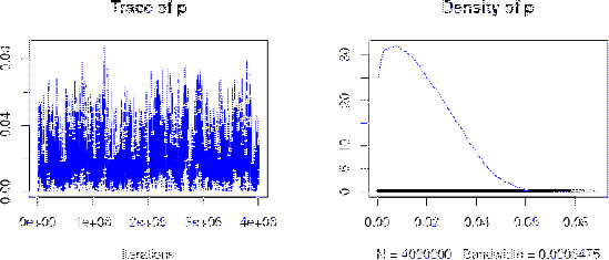It is true that, if there were no infected in the population, then we would expect $n_P \approx 1150$ (with a standard uncertainty of 220), but the distribution of $p$ provided by the inference cannot have a mean value zero, simply because negative values of $p$ are impossible.⁵¹Obviously the smaller is the number of positives in the sample and more peaked is the distribution of $p$ close to 0. But what happens if, for $n_s=10000$, $n_P$ is much smaller of 1150? This interesting case will be the subject of the next subsection.