Using the R random number generators
The implementation in R is rather simple, thanks
also to the capability of the language to handle `vectors', meant
as one dimensional arrays, in a compact way. The steps described above
can then be implemented into the following
lines of code:
n.I   <- rbinom(nr, ns, p)       # 1.
n.NI  <- ns - n.I
pi1   <- rbeta(nr, r1, s1)       # 2.
pi2   <- rbeta(nr, r2, s2)
nP.I  <- rbinom(nr, n.I, pi1)    # 3.
nP.NI <- rbinom(nr, n.NI, pi2)
nP    <- nP.I + nP.NI            # 4.
We just need to define the parameters of interest,
including nr, number of extractions, run
the code and add other instructions in order
to print and plot the results (a minimalist script performing all tasks
is provided in Appendix B.5). The only instructions
worth some further comment are the two related to the step nr. 3.
A curious feature of the `statistical functions' of R
is that they can accept vectors for the number of trials and for
probability at each trial, as it is done here. It means that
internally the random generator is called nr times,
the first time e.g. with n.I 1
1![$]$](img65.png) and pi11, the second time with
n.I2 and pi12, and so on, thus
avoiding us to use explicit loops.
Note that, if precise values of
and pi11, the second time with
n.I2 and pi12, and so on, thus
avoiding us to use explicit loops.
Note that, if precise values of  and
and  were assumed,
then we just need to replace the two lines of step nr. 2
with the assignment of their numeric values.
were assumed,
then we just need to replace the two lines of step nr. 2
with the assignment of their numeric values.
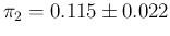
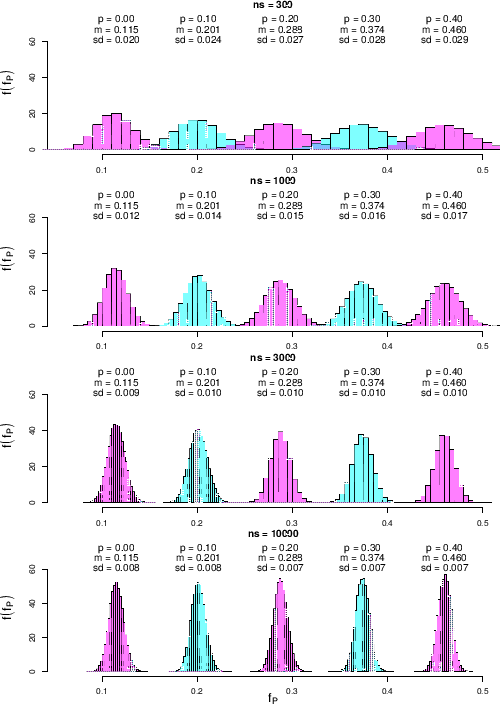
Figure ![[*]](crossref.png) shows the results
shows the results
Figure:
Predictive distributions of  as a function of
  and
and  for our default
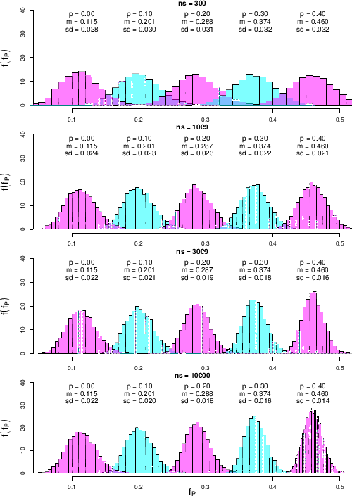
uncertainty on , summarized as
for our default
uncertainty on , summarized as
 .
.
 |
obtained for some values of and , and modeling the
uncertainty of and in our default way,
summarized by
 and
.
The values of have been chosen in steps of roughly
half order of magnitude
in the region of
and
.
The values of have been chosen in steps of roughly
half order of magnitude
in the region of  of interest,
as we have learned in Sec. .
We see that
for the smallest shown in the figure, equal to 300,
varying by 0.1 produces distributions of with
quite some overlap. Therefore with samples of such a small
size we can say, very qualitatively that we
can resolve different values of if they do not
differ less than
of interest,
as we have learned in Sec. .
We see that
for the smallest shown in the figure, equal to 300,
varying by 0.1 produces distributions of with
quite some overlap. Therefore with samples of such a small
size we can say, very qualitatively that we
can resolve different values of if they do not
differ less than
 . The situations improves
(the separation roughly doubles)
when we increase to 1000 or even to 3000, while there is no further
gain reaching
. The situations improves
(the separation roughly doubles)
when we increase to 1000 or even to 3000, while there is no further
gain reaching  . This is in agreement with what
we have learned in the previous section.
. This is in agreement with what
we have learned in the previous section.
Since, as we have already seen, the limiting effect is due to
systematics, and in particular, in our case, to the uncertainty
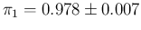
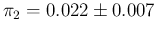
about , we show in Fig.
Figure:
Same as Fig. , but for
an improved knowledge of , summarized as
 .
.
 |
how the result changes if we reduce
 to the level
of
to the level
of
 .39As we can see (a result largely expected), there is quite
a sizable improvement
in separability of values of for large values of .
Again qualitatively, we can see that values of
which differ by
.39As we can see (a result largely expected), there is quite
a sizable improvement
in separability of values of for large values of .
Again qualitatively, we can see that values of
which differ by
 can be resolved.
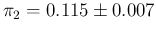
Finally we show in Fig.
Figure:
Same as
Fig. , but for
an improved specificity, summarized as
 .
.
 |
the case in which sensitivity and specificity are equal, both
as expected value and standard uncertainty. The first thing we note in these new
histograms is that for  they are no longer symmetric and
Gaussian-like. This is due to the fact that no negative values of
they are no longer symmetric and
Gaussian-like. This is due to the fact that no negative values of  are possible, and then there is a kind of `accumulation'
for low values of , and therefore of
(this kind of skewness is typical of all probability distributions
of variables defined to be positive and whose standard deviation is not
much smaller than the expected value - think e.g.
at a Poissonian with
are possible, and then there is a kind of `accumulation'
for low values of , and therefore of
(this kind of skewness is typical of all probability distributions
of variables defined to be positive and whose standard deviation is not
much smaller than the expected value - think e.g.
at a Poissonian with  ).
).