Next: Normalization factor and other Up: Exact evaluation of Previous: Exact evaluation of Contents
![[*]](crossref.png) , the inference
of the `unobserved' variables, based on the `observed' one,
for the problem represented graphically in the `Bayesian'
network of Fig. , consists
in evaluating `somehow'
) is proportional to Eq. (),
hereafter indicated by `:
, the inference
of the `unobserved' variables, based on the `observed' one,
for the problem represented graphically in the `Bayesian'
network of Fig. , consists
in evaluating `somehow'
) is proportional to Eq. (),
hereafter indicated by `:
 d d |
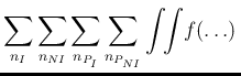
As a first step we simplify the equation by summing
over
![]() and
and ![]() and exploiting the Kroneker delta
terms () and ().
We can then replace
and exploiting the Kroneker delta
terms () and ().
We can then replace
![]() with
with
![]() and
and ![]() with
with ![]()
 |
(96) |
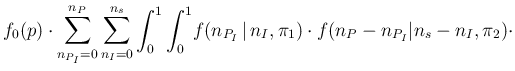
The inferential distribution of interest
![]() ,
becomes then, besides constant factors and indicating
all the status of information on which the inference is based
as `
,
becomes then, besides constant factors and indicating
all the status of information on which the inference is based
as `![]() ', that is
', that is
![]() ,
,
 |
|||
 |
|||
 |
|||
 d d |
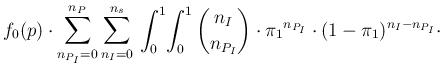
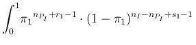
The two integrals appearing
in Eq. () are, in terms of the generic variable ![]() ,
of the form
,
of the form
![]() d
d![]() ,
which defines the special function beta
B
,
which defines the special function beta
B![]() ,
whose value
can be expressed
in terms of Gamma function as
B
,
whose value
can be expressed
in terms of Gamma function as
B![]() .
We get then
.
We get then
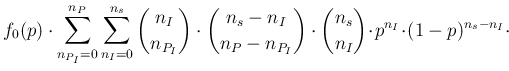
 d
d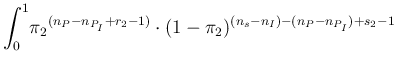 d
d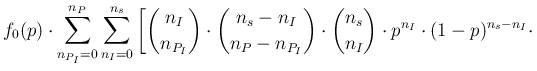
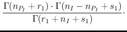
![$\displaystyle \left.\frac{\Gamma (n_P-n_{P_I}+r_2)\cdot \Gamma(n_s-n_I-n_P+n_{P_I}+s_2)}
{ \Gamma(n_s-n_I+s_2+r_2)} \right] \,.$](img903.png)