Predicting the fractions of positives obtained sampling two different populations

An interesting question then arises: what happens if we measure, using tests having the same uncertainties on sensitivity and specificity, two different populations, having proportions of infectees $p^{(1)}$ and $p^{(2)}$, respectively? For example, in order to make use of results we have got above, let us take the results shown in Fig.  for $n_s=10000$, $p^{(1)}=0.1$ and $p^{(2)}=0.2$. For this value of the sample size and for our standard hypotheses for sensitivity and specificity, summarized as $\pi_1=0.978\pm 0.007$ and $\pi_2=0.115\pm 0.022$, the uncertainties are dominated by the systematic contributions. Our expectations are then $f_P^{(1)} = 0.201\pm 0.020$ and $f_P^{(2)} = 0.288\pm 0.018$. The difference of expectations is therefore $\Delta f_P = f_P^{(2)} - f_P^{(1)} = 0.087$.

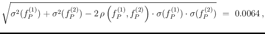
Now it is interesting to know how much uncertain this number is. One could improperly use a quadratic combination of the two standard uncertainties, thus getting $\Delta f_P = 0.087 \pm 0.027$. But this evaluation of the uncertainty on the difference is incorrect because $f_P^{(1)}$ and $f_P^{(2)}$ are obtained from the same knowledge of $\pi_1$ and $\pi_2$, and are therefore correlated. Indeed, in the limit of negligible uncertainties on these two parameters, the expectations would be much more precise, as we can see from the upper plot of Fig. , with a consequent reduction of $\sigma(\Delta f_P)$. These are the results, obtained by Monte Carlo evaluation using only R commands (see script in Appendix B.8),⁴³with one extra digit with respect to Fig.  and adding also the correlation coefficient:

$$f_P^{(1)} = 0.2013 \pm 0.0199$$

$$f_P^{(2)} = 0.2876 \pm 0.0179$$

$$\Delta f_P = 0.0863 \pm 0.0064$$

$$\rho\left(f_P^{(1)},f_P^{(2)}\right) = 0.9470$$

The uncertainty on $\Delta f_P$ is about one fourth of what naively evaluated above and about one third of the individual predictions, due to the well known effect of (at least partial) cancellations of uncertainties in differences, due to common systematic contributions. In this case, in fact, the standard deviation of $\Delta f_P$, calculated from standard deviations and correlation coefficient, is given by⁴⁴

$$\sigma(\Delta f_P) = \sqrt{\sigma^2(f_P^{(1)}) + \sigma^2(f_P^{(2)}) - 2\,\rho\left(f_... ...(2)}\right)\cdot \sigma(f_P^{(1)})\cdot \sigma(f_P^{(2)}) }\,\, = \,\,0.0064\,,$$

in perfect agreement with what we get from Monte Carlo sampling.

An important consequence of the correlation among the predictions of the numbers of positives in different populations is that we have to expect a similar correlation in the inference of the proportion of infectees in different populations. This implies that we can measure their difference much better than how we can measure a single proportion. And, if one of the two proportions is precisely known using a different kind of test, we can take its value as kind of calibration point, which will allow a better determination also of the other proportion. We shall return to this interesting point in Sec. .