Having to turn the qualitative judgment regarding the `separation'
of the distributions of  for different
  , as it results
from
Figs.
, as it results
from
Figs. ![[*]](crossref.png) -,
into a resolution power, one needs some convention.
First, we remind that, unless is very small,
we have good theoretical reasons, confirmed by Monte Carlo
simulations, that
-,
into a resolution power, one needs some convention.
First, we remind that, unless is very small,
we have good theoretical reasons, confirmed by Monte Carlo
simulations, that  is about Gaussian, at least in the
range of a few standard deviations around its mean value.
But Gaussian curves are, strictly speaking, never separated from
each other, because they have as domain the entire
real axis for all
is about Gaussian, at least in the
range of a few standard deviations around its mean value.
But Gaussian curves are, strictly speaking, never separated from
each other, because they have as domain the entire
real axis for all  's and
  's.
In fact this is a “defect” of such
distribution,
as Gauss himself called it [9] and some grain of salt
is required using it.
In order to form an idea of how one could define conventionally
`resolution', the upper plot of
Fig. shows
's.
In fact this is a “defect” of such
distribution,
as Gauss himself called it [9] and some grain of salt
is required using it.
In order to form an idea of how one could define conventionally
`resolution', the upper plot of
Fig. shows
Figure:
Upper plot: Examples of Gaussians whose parameters
are separated by 1 . Bottom plot:
resolution power in , defined by Eq. (),
for  (lines between points just to guide the eye).
Filled (blue) circles for
(lines between points just to guide the eye).
Filled (blue) circles for  and open (cyan) circles for
  .
Solid lines for
.
Solid lines for
 , dashed lines for
 and dotted lines for
 (
(
 in all cases).
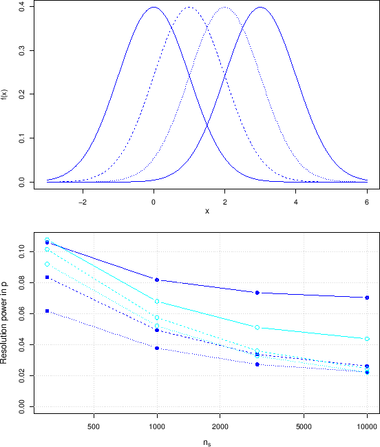 |
some Gaussians having unitary , with 's differing
by one  .
.
We see that a `reasonable separation' is achieved
when they differ by a few 's - let us say, generally
speaking,
 , although absolute separation
can never occur, for the already quoted intrinsic “defect” of the distribution.
Having to choose a value, we just
opt arbitrarily for , corresponding to the
two solid lines of the figure, although the
conclusions that follow from this choice can be easily
rescaled at wish.
Moreover, as we can see from
Figs. -
(and as it results from the approximated formulae)
, although absolute separation
can never occur, for the already quoted intrinsic “defect” of the distribution.
Having to choose a value, we just
opt arbitrarily for , corresponding to the
two solid lines of the figure, although the
conclusions that follow from this choice can be easily
rescaled at wish.
Moreover, as we can see from
Figs. -
(and as it results from the approximated formulae)
- the standard deviation of the distributions varies
smoothly with ;
- the mean value depends linearly on
for obvious reasons.42
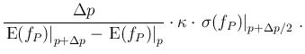
Therefore the resolution power in the interval
![$[p,p+\Delta p]$](img607.png) can be
evaluated by a simple proportion
can be
evaluated by a simple proportion
For example, using the numbers of the Monte Carlo evaluations
shown in Fig. ,
for and  we get
 ,
reaching at best
,
reaching at best
 in the case of
  shown in
Fig. .
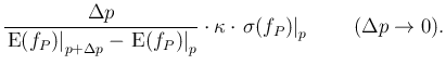
The resolution power at a given value of , is obtained
in the limit `
shown in
Fig. .
The resolution power at a given value of , is obtained
in the limit `
 ':
':
The bottom plot of Fig.
shows the variation of the resolution power in
for the same
values of  of
Figs. -
and for the usual cases of
of
Figs. -
and for the usual cases of  and
and  of those
figures (in the order: solid, dashed and dotted line -
the lines are drawn just
to guide the eye and to easily identify the conditions).
The resolution power has been evaluated using the approximated
formulae, for , around
(blue filled circles) and around
(cyan open circles),
using for the gradient
of those
figures (in the order: solid, dashed and dotted line -
the lines are drawn just
to guide the eye and to easily identify the conditions).
The resolution power has been evaluated using the approximated
formulae, for , around
(blue filled circles) and around
(cyan open circles),
using for the gradient
 (the exact value
is irrelevant for the numerical evaluation, provided
it is small enough).
(the exact value
is irrelevant for the numerical evaluation, provided
it is small enough).
 Obviously, if one prefers a different value
of
Obviously, if one prefers a different value
of  (in particular one might like
  ), then
one just needs to rescale the results.
), then
one just needs to rescale the results.![$]$](img65.png)