Equation (![[*]](crossref.png) ) is
a straight consequence of the probability rule relating
joint probability to conditional probability, that is,
for the generic `events'
) is
a straight consequence of the probability rule relating
joint probability to conditional probability, that is,
for the generic `events'  and
and  ,
,
having added to
 Inf
Inf of Eq. ()
the suffix `0' in order to emphasize its
role of `prior' probability.
Equation (A.1) yields trivially
of Eq. ()
the suffix `0' in order to emphasize its
role of `prior' probability.
Equation (A.1) yields trivially
having also emphasized that  in r.h.s. is the probability
of before it is updated by the new condition
.59But, indeed, the essence of the Bayes' rule is given by
in r.h.s. is the probability
of before it is updated by the new condition
.59But, indeed, the essence of the Bayes' rule is given by
in which we have rewritten the ` ' in the way it is
custom for uncertain numbers (`random variables'),
as we shall see in while. Moreover, as we can `expand' the numerator
(using the so called chain rule)
to go from Eq. (A.3) to Eq. (A.2), and then
Eq. (), similarly we can
expand the denominator in two steps.
We start `decomposing' into
' in the way it is
custom for uncertain numbers (`random variables'),
as we shall see in while. Moreover, as we can `expand' the numerator
(using the so called chain rule)
to go from Eq. (A.3) to Eq. (A.2), and then
Eq. (), similarly we can
expand the denominator in two steps.
We start `decomposing' into  and
and
 ,
from which it follows
,
from which it follows
After the various `expansions' we can rewrite Eq. (A.3) as
Finally, if instead of only two possibilities and
 , we have a complete class of hypotheses
  ,
i.e. such that
,
i.e. such that
 and
and
 for
for  ,
we get the famous
,
we get the famous
having also replaced the symbol by  , given its meaning
of effect, upon which the probabilities of
the different hypotheses are updated.
Moreover, the sum in the denominator of the first
r.h.s. of Eq. (A.5) makes it explicit that the
denominator is just a normalization factor, and therefore the
essence of the reasoning can be expressed as
, given its meaning
of effect, upon which the probabilities of
the different hypotheses are updated.
Moreover, the sum in the denominator of the first
r.h.s. of Eq. (A.5) makes it explicit that the
denominator is just a normalization factor, and therefore the
essence of the reasoning can be expressed as
The extension to discrete `random variables' is straightforward,
since the probability distribution  has the meaning
of
has the meaning
of  , with
  the name of the variable and
 one of the possible values that it can assume.
Similarly,
one of the possible values that it can assume.
Similarly,  stands for
 ,
,
 for
for
 , and so on.
Moreover all possible values of , as well as all possible
values of
, and so on.
Moreover all possible values of , as well as all possible
values of  , form a complete class of hypotheses
(the distributions are normalized). Equation (A.3)
and its variations and `expansions' becomes then, for and ,
, form a complete class of hypotheses
(the distributions are normalized). Equation (A.3)
and its variations and `expansions' becomes then, for and ,
which can be further extended to several other variables.
For example,
adding  ,
,  and
and  and being interested to the joint
probability that and assume the values and
and being interested to the joint
probability that and assume the values and  ,
conditioned by
,
conditioned by  ,
,  and
and  , we get
To conclude, some remarks are important, especially for the applications:
- Equations (A.7) and (A.8) are valid also for continuous variables,
in which case the various `
 ' have the meaning of
probability density function, and the sums needed to get
the (possibly joint) marginal in the
denominator are replaced by integration.
' have the meaning of
probability density function, and the sums needed to get
the (possibly joint) marginal in the
denominator are replaced by integration.
- The numerator of Eq. (8)
is `expanded' using a chain rule,
choosing, among the several possibilities, that which
makes explicit the
(assumed) causal connections60of the different variables in the game, as stressed in the proper
places through the paper (see e.g. footnote ,
Sec. and Sec. ).
- A related remark is that, among the variables entering the game,
as those of Eq. (A.8), some may be continuous
and other discrete and the probabilistic meaning of `
 ',
taking the example of
a bivariate case with discrete and
',
taking the example of
a bivariate case with discrete and
 continuous, is given by
 d
d d,
with the normalization condition
given by
d,
with the normalization condition
given by
 d
d .
.
- Finally, a crucial observation is that, given the model
which connects the variables (the graphical representations
of the kinds shown in the paper are very useful to understand it)
and its parameters, the denominator of Eq. (A.8)
is just a number
(although often very difficult to evaluate!),
and therefore, as we have seen in Eq. (A.7),
the last equation can be rewritten as

or, denoting by
 the un-normalized
posterior distribution,
the un-normalized
posterior distribution,
The importance of this remark is that, although a closed
form of posterior is often prohibitive in practical cases,
an approximation of it
can be obtained by Monte Carlo techniques,
which allow us to evaluate the quantities of interest,
like averages, probability intervals, and so on
(see references in footnote ).
---------------------------------------------------
 (A.2)
(A.2)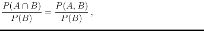 (A.3)
(A.3)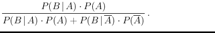 (A.4)
(A.4)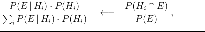 (A.5)
(A.5)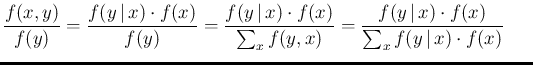
 (A.8)
(A.8)![$\displaystyle \frac{1}{2\,\pi\,\sigma_x\,\sigma_y\,\sqrt{1-\rho^2}}\,
\exp \lef...
...u_y)}{\sigma_x\,\sigma_y}
+ \frac{(y-\mu_y)^2}{\sigma_y^2}
\right]
\right\} \,.$](img1026.png)
![$\displaystyle \frac{1}{2\,\pi\,\sigma_x\,\sigma_y\,\sqrt{1-\rho^2}}\,
\exp \lef...
...\mu_y)}{\sigma_x\,\sigma_y}
+ \frac{(y_0-\mu_y)^2}{\sigma_y^2}
\right]
\right\}$](img1029.png)
![$\displaystyle \exp \left\{
-\frac{1}{2\,(1-\rho^2)}
\left[ \frac{(x-\mu_x)^2}{\sigma_x^2}
- 2\,\rho\,\frac{x\,(y_0-\mu_y)}{\sigma_x\,\sigma_y}
\right]
\right\}$](img1030.png)
![$\displaystyle \exp \left\{
-\frac{1}{2\,(1-\rho^2)\,\sigma_x^2}
\left[x^2 -2\,x\,\left(\mu_x+\rho\frac{\sigma_x}{\sigma_y}\,
(y_0-\mu_y)\right)
\right]
\right\}$](img1031.png)
![$\displaystyle \exp \left\{-\frac{\left[x^2 -2\,x\,\left(\mu_x+\rho\frac{\sigma_x}{\sigma_y}\,
(y_0-\mu_y)\right)
\right]}
{2\,(1-\rho^2)\,\sigma_x^2}
\right\}$](img1032.png)
![$\displaystyle \exp \left\{-\frac{\left[x -\,\left(\mu_x+\rho\frac{\sigma_x}{\sigma_y}\,
(y_0-\mu_y)\right)
\right]^2}
{2\,(1-\rho^2)\,\sigma_x^2}
\right\} \,,$](img1033.png)
 at the exponent is the same as multiplying by a constant factor.