Standard combination from a probabilistic perspective

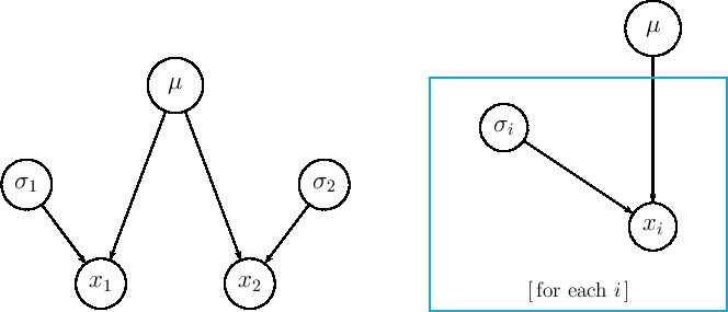
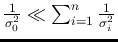
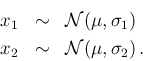
Let us start with just two experimental outcomes,¹⁰ $x_1$ and $x_2$, resulting from the uncertain `true' value $\mu$ (what we are interested in) when measured in two independent experiments having Gaussian error functions with standard deviations $\sigma_1$ and $\sigma_2$, as sketched in the left hand graph of Fig. 5.

Figure: Graphical model behind the standard combination.

That is

$$\begin{eqnarray*} x_1 &\sim & {\cal N}(\mu, \sigma_1)\\ x_2 &\sim & {\cal N}(\mu, \sigma_2)\,. \end{eqnarray*}$$

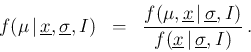
The general case, with many measurements of the same $\mu$, is shown on the right hand graph of the same figure. From a probabilistic point of view our aim will be to assess, with a probability distribution, the intervals where we believe $\mu$ lies with different probabilities, that is to arrive to

$$\begin{eqnarray*} f(\mu\,\vert\,x_1,x_2,\ldots,\sigma_1,\sigma_2,\ldots,I) \equiv f(\mu\,\vert\,\underline{x},\underline{\sigma}\ldots,I). \end{eqnarray*}$$

The pdf of interest can be (in principle) obtained easily if we knew the joint pdf of all the quantities of interest, that is $f(\mu,\underline{x}\,\vert\,\underline{\sigma},I)$. In fact, we just need to apply a well know general rule of probability theory (remember that in this first example the $\sigma_i$ are just fixed conditions, although in general they might become subject to inference too, as we shall see later):

$$\begin{eqnarray*} f(\mu\,\vert\,\underline{x},\underline{\sigma},I) &=& \frac{... ...{\sigma},I)} {f(\underline{x}\,\vert\,\underline{\sigma},I)}\,. \end{eqnarray*}$$

At this point the reader might be scared by two reasons: the first is how to build up the joint pdf $f(\mu,\underline{x}\,\vert\,\underline{\sigma},I)$; the second is how to perform the integral over $\mu$ (`marginalization') in order to get the denominator.¹¹

The first good news is that, given the model (those of Fig. 5 or the more complicate ones we shall see later), the denominator is just a number, in general difficult to calculate, but just a number. This means that we can rewrite the previous equation as

$$f(\mu\,\vert\,\underline{x},\underline{\sigma},I) \propto f(\mu,\underline{x}\,\vert\,\underline{\sigma},I)\,.$$ (3)

As next step, we can follow two strategies:

• calculate the normalization factor at the end, either analytically or numerically;
• sample the unnormalized distribution by Monte Carlo techniques, in order to get the shape of $f(\mu\,\vert\,\underline{x},\underline{\sigma},I)$ and to calculate all moments of interest.

The second good news is that the multidimensional joint pdf can be easily written down using the well known probability theory theorem known as chain rule. Indeed, sticking to the model with just two variables, we can apply the chain rule in different ways. For example, beginning from the most pedantic one, we have

$$\begin{eqnarray*} f(\mu,x_1,x_2\,\vert\,\sigma_1,\sigma_2,I) &=& f(\mu\,\vert... ...sigma_1,\sigma_2,I) \cdot f(x_2\,\vert\,\sigma_1,\sigma_2,I)\,. \end{eqnarray*}$$

But this writing does not help us, since it requires $f(\mu\,\vert\,x_1,x_2,\sigma_1,\sigma_2,I)$, which it is precisely what we aim for. It is indeed much better, with an eye to Fig. 5, a bottom up approach (in the following equation the order of the arguments in the left side term has been changed to make the correspondence between the two writings easier), that is

$$\begin{eqnarray*} f(x_1,x_2,\mu,\,\vert\,\sigma_1,\sigma_2I) & = & f(x_1\,\ver... ...igma_1,\sigma_2,I) \cdot f(\mu\,\vert\,\sigma_1,\sigma_2,I)\,. \end{eqnarray*}$$

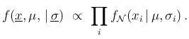
This equation can be further simplified if we note that each $x_i$ depends directly only on $\mu$ and $\sigma_i$, while $\mu$ does not depend (at least in usual measurements) on $\sigma_1$ and $\sigma_2$. We get then

$$f(x_1,x_2,\mu,\,\vert\,\sigma_1,\sigma_2,I) = f(x_1\,\vert\,\mu,\sigma_1,I) \cdot f(x_2\,\vert\,\mu,\sigma_2,I) \cdot f(\mu\,\vert\,I)\,.$$ (4)

We can easily generalize this equation, in the case of many observations described in the right hand graph of Fig. 5, rewriting it as

$$f(\underline{x},\mu,\,\vert\,\underline{\sigma}) = \left[ \prod_i f(x_i\,\vert\,\mu,\sigma_i)\right]\cdot f_0(\mu)$$ (5)

where the index $i$ runs through all the observations and the symbol `$I$' indicating the background state of information has been dropped, using `$f_0(\mu)$' for the initial distribution (`prior') of $\mu$. Finally, taking (for the moment) for $f_0(\mu)$ a practically flat distribution in the region of interest (see footnote 9), making use of Eq. (3) and of the symbol $f_{\cal N}$ to indicate normal (i.e. Gaussian) error functions, we get

$$f(\mu\,\vert\,\underline{x},\underline{\sigma},f_0(\mu)=k) \propto f(\underline{x},\mu,\,\vert\,\underline{\sigma}) \ \propto \ \prod_i f_{{\cal N}}(x_i\,\vert\,\mu,\sigma_i)\,.$$ (6)

Using the explicit expression of the Gaussian and neglecting all multiplicative factors that do not depend on $\mu$, we get

$$f(\mu\,\vert\,\underline{x},\underline{\sigma},f_0(\mu)=k) \propto \prod_i \exp\left[-\frac{(x_i-\mu)^2}{2\,\sigma_i^2}\right]$$ (7)

$$\propto \exp\left[-\sum_i\,\frac{(x_i-\mu)^2}{2\,\sigma_i^2}\right]$$

$$\propto \exp\left[-\frac{1}{2} \sum_i\,\frac{x_i^2-2 x_i \mu + \mu^2}{\sigma_i^2} \right]$$

$$\propto \exp\left[-\frac{1}{2} \sum_i\,\left(\frac{x_i^2}{\sigma_i^2}-2\, \frac{x_i}{\sigma_i^2}\, \mu + \frac{\mu^2}{\sigma_i^2}\right) \right]$$

$$\propto \exp\left[-\frac{1}{2}\cdot \frac{\sum_i 1/\sigma_i^2}{\sum_i 1/\... ...2}\right)\, \mu + \left(\sum_i\frac{1}{\sigma_i^2}\right) \mu^2 \right) \right]$$

$$\propto \exp\left[-\frac{1}{2}\cdot \left(\sum_i 1/\sigma_i^2\right) \cdot\left( \overline{x^2} - 2\,\overline{x}\,\mu + \mu^2 \right) \right]$$

$$\propto \exp\left[- \frac{ \overline{x^2} - 2\,\overline{x}\,\mu + \mu^2}{2/(\sum_i 1/\sigma_i^2)} \right]$$ (8)

$$\propto \exp\left[- \frac{ - 2\,\overline{x}\,\mu + \mu^2}{2\,\sigma_C^2} \right] \,,$$ (9)

where

$$\overline{x} = \frac{\sum_i\,x_i/\sigma_i^2} {\sum_i 1/\sigma_i^2}$$ (10)

$$\overline{x^2} = \frac{\sum_i\,x_i^2/\sigma_i^2} {\sum_i 1/\sigma_i^2}$$

$$\sigma_C^2 = \frac{1}{\sum_i 1/\sigma_i^2}\,.$$ (11)

Note that the mean of the squares $\overline{x^2}$ has been taken out of the exponent $[$ step from Eq. (8) to Eq. (9) $]$ because $\exp[-\overline{x^2}/(2\sigma_C^2)]$ does not depend on $\mu$ and therefore it can be absorbed in the normalization constant. For the same reason we can multiply Eq. (9) by $\exp[-\overline{x}^2/(2\sigma_C^2)]$, thus getting, by complementing the exponential,

$$\begin{eqnarray*} f(\mu\,\vert\,\underline{x},\underline{\sigma},f_0(\mu)=k) &\... ...\left[- \frac { (\mu-\overline{x})^2} {2\,\sigma_C^2} \right] \end{eqnarray*}$$

We can now recognize in it, at first sight, a Gaussian distribution of the variable $\mu$ around $\overline{x}$, with standard deviation $\sigma_C$, i.e.

$$f(\mu\,\vert\,\underline{x},\underline{\sigma},f_0(\mu)=k) = \frac{1}{\sqrt{2\,\pi}\,\sigma_C}\, \exp\left[- \frac { (\mu-\overline{x})^2} {2\,\sigma_C^2} \right]$$ (12)

with expected value $\overline{x}$ and standard deviation $\sigma_C$.

Someone might be worried about the dependence of the inference on the flat prior of $\mu$, written explicitly in Eq. (12), but what really matters is that $f_0(\mu)$ does not vary much in the region of a few $\sigma_C$'s around $\overline{x}$. Since in the software package that we are going to use, starting from next section, an explicit prior is required, let us try to understand the influence of a vague but not flat prior in the resulting inference. Let us model $f_0(\mu)$ with a Gaussian distribution having a rather large $\sigma_0$ (e.g. $\sigma_0 \gg \sigma_i$) and centered in $x_0 \approx {\cal O}(x_i)$. The result is that Eq. (7) becomes

$$f(\mu\,\vert\,\underline{x},\underline{\sigma}) \propto \prod_i \exp\left[-\frac{(x_i-\mu)^2}{2\,\sigma_i^2}\right]\cdot \exp\left[-\frac{(\mu-x_0)^2}{2\,\sigma_0^2}\right]\,.$$ (13)

This is equivalent to add the extra term $x_0$ with standard uncertainty $\sigma_0$, which has then to be included in the calculation of $\overline{x}$ and $\sigma_C$ $[$technically the index $i$ in the sums in Eqs. (10) and (11) run from 0 to $n$, instead than from $1$ to $n$, being $n$ the number of measurements$]$. But if $\sigma_0 \gg \sigma_i$ (more precisely $\frac{1}{\sigma_0^2} \ll \sum_{i=1}^n\frac{1}{\sigma_i^2}$) and $x_0$ is `reasonable', then the extra contribution is irrelevant.