Introduction

It is not rare the case in which experimental results `appear' to be in mutual disagreement. The quote marks are mandatory, as a reminder that also very improbable events might by nature occur.¹The fact that they `appear' to us in mutual disagreement is because we know by experience that uncertainties²might be underestimated, systematic errors overlooked, theoretical corrections not (properly) taken into account, or even mistakes of different kinds having possibly been made in building/running the experiment or in the data handling. It is enough to browse the PDG [3] to find cases of this kind, as the one of Fig. 1 concerning the mass of the charged kaon, whose values, as selected by the PDG,

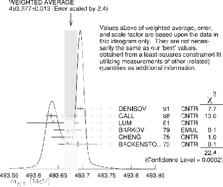
**Figure:** Charged kaon mass from several experiments as summarized by the PDG [3]. Note that besides the `error' of 0.013 MeV, obtained by a $\times 2.4$ scaling, also an `error' of 0.016 MeV is provided, obtained by a $\times 2.8$ scaling. The two results are called `OUR AVERAGE' and 'OUR FIT', respectively.
$\begin{figure}\centering\epsfig{file=PDG_summary.eps,clip=,width=0.8\linewidth}\end{figure}$

are reported in Tab. 1.³

Table: Experimental values of the charged kaon mass, limited to those taken into account by the 2019 issue of PDG [3] (see footnote 3 for remarks).

Authors	pub. year	central value	uncertainty
		(MeV)	(MeV)
G. Backenstoss et al. [4]	1973	493.691	0.040
S.C. Cheng et al. [5]	1975	493.657	0.020
L.M. Barkov et al.[6]	1979	493.670	0.029
G.K. Lum et al. [7]	1981	493.640	0.054
K.P. Gall et al. [8]	1988	493.636	0.011 (*)
A.S. Denisov et al. [9]	1991	493.696	0.0059
& Yu.M. Ivanov [10]	1992	same	0.007

The usual probabilistic interpretation⁴of the results is that each experiment provides a probability density function (pdf) centered in with standard deviation , as shown by the solid lines of Fig. 2.

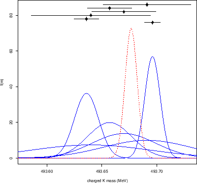
**Figure:** *Graphical representation of the results on the charged kaon mass of Tab. 1 (solid lines). The dashed red Gaussian shows the result of the* *naive* standard combination (see text).
$\begin{figure}\centering\epsfig{file=naive_combination.eps,clip=,width=0.76\linewidth}\end{figure}$

The standard way to combine the individual results consists in calculating the weighted average, with weights equal to

, that is

$\displaystyle d_w$	$\textstyle =$	$\displaystyle \frac{\sum_id_i/s_i^2}{\sum_i1/s_i^2}$	(1)
$\displaystyle s_w$	$\textstyle =$	$\displaystyle \left(\sum_i1/s_i^2\right)^{-\frac{1}{2}}\,,$	(2)

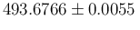which, applied to the values of Tab. 1, yields $d_w = 493.6766\,$ MeV and $s_w = 0.0055\,$ MeV, i.e. a charged kaon mass of $493.6766\pm 0.0055\,$ MeV,⁵ graphically shown in Fig. 2 with a dashed red Gaussian. The outcome `appears' suspicious because the probability mass is concentrated in the region less preferred by the individual more precise results, as also emphasized in the ideogram of Fig. 1, on the meaning of which we shall return in section 5.

As a matter of fact, a situation of this kind is not impossible, but nevertheless, there is a natural tendency to believe that there must be something not properly taken into account by one or more experiments. Told with a dictum attributed to a famous Italian politician, “a pensar male degli altri si fa peccato ma spesso ci si indovina”.⁶

**Figure:** *Same as Fig. 2 but with one result* *arbitrarily* shifted by $-50\,$ keV (dotted line).
$\begin{figure}\centering\epsfig{file=naive_combination_Andreotti.eps,clip=,width=0.8\linewidth}\end{figure}$

For example, looking at Fig. 2, one is strongly tempted to lower, just as an exercise, the highest value by 50 keV,⁷thus getting the excellent overall agreement shown in Fig. 3 (shifted Gaussian plotted with a dotted gray line), yielding a combined mass value of 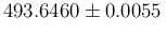$493.6460 \pm 0.0055\,$ MeV. And the question would be settled. But this sounds at least unfair. In particular because we are aware, from the history of measurements, of a kind of `inertia' of new results to different from old ones - but sometimes the new results moved `too far' from the old ones and the presently accepted value lies somewhere in the middle.

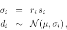
**Figure:** *Some history plots from the PDG [3,14].*
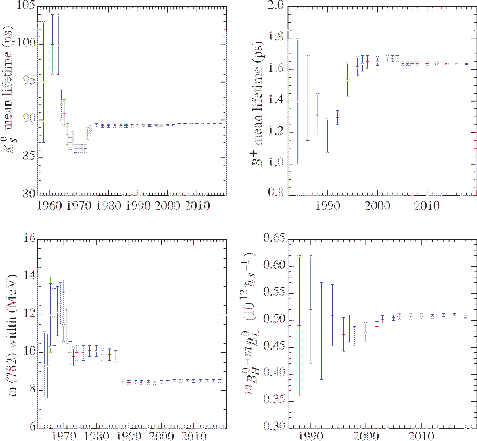$\begin{figure}\centering\epsfig{file=history_plot_UR.eps,clip=,width=0.87\linewidth}\end{figure}$

Figure 4 shows some of the history plots traditionally reported by the PDG [14].

In such a state of uncertainty, probability theory can help us in building up a model in which the values about which we are in doubt are allowed to vary from the nominal ones. Obviously, the model is not unique, as not unique are the probability distributions that can be used. Following then [15], inspired to [16], these are the criteria followed and some (hopefully shareable) desiderata:

the quantities on which we focus our doubts are the reported uncertainties , assumed to have the meaning of standard uncertainty [1,2], as commented above;⁸
the `true' standard deviations $\sigma_i$ are related to by a factor (one for each experiment), i.e.

$\begin{eqnarray*} \sigma_i &=& r_i\,s_i \\ d_i &\sim & {\cal N}(\mu, \sigma_i)\,, \end{eqnarray*}$

where the last notation means that is described by a Gaussian (`normal') distribution centered on the `true' value of the quantity of interest, generically indicated by $\mu$ , with standard deviation $\sigma_i$ ;
all experiments are treated democratically and fairly, i.e. our prior belief of each has expected value equal to 1, and its prior distribution does not depend on the experiment:

$\begin{eqnarray*} f(r_1\,\vert\,I) &=& f(r_2\,\vert\,I)\ = \ f(r_3\,\vert\,I)\ =\ \cdots \\ \mbox{E}[r_i\,\vert\,I] &=& 1\,, \end{eqnarray*}$

where `' stands for the background status of information (probability is always conditional probability!);
but we are sceptical, and hence each has Ã priori a wide range of possibilities described by a suitable (easy to handle) probability distribution, the details of which will be give later - we just anticipate that we take a prior 100% standard uncertainty on , i.e. $\sigma(r_i\,\vert\,I)/\mbox{E}[r_i\,\vert\,I]=1$ ;
one of the desiderata of the model is that the posterior pdf of the physical quantity of interest should not be limited to a Gaussian and could even be multimodal if the individual results cluster in different regions; or it could be narrower than the pdf obtained by the standard weighted average, if the individual results tend to overlap `too much' (see e.g. Figs. 4 and 5 of Ref. [15]);
finally, once the parameters of $f(r_i\,\vert\,I)$ are defined on bench marks and checked against `reasonable' variation (as done in Figs. 4 and 5 of Ref. [15]), fine tuning and cherry peaking of the individual results to be included in the combination should be avoided (unless we have good reasons to mistrust some results).

Once the model has been built, we can easily write down the multidimensional probability pdf $f(\underline{d},\mu,\underline{r}\,\vert\,\underline{s},I)$ , of all the variables of interest (the `observed'

and the uncertain values $\mu$ and

's - the

will be instead considered as fixed conditions, as it will be clear in a while; $\underline{d}$ stands for all the

, and so on).

Once the multi-dimensional pdf has been settled, writing down the unnormalized pdf of the uncertain quantities,

$\begin{eqnarray*} \widetilde{f}(\mu,\underline{r}\,\vert\,\underline{d},\underl... ...& f(\mu,\underline{r}\,\vert\,\underline{d},\underline{s},I)\,, \end{eqnarray*}$

is straightforward, as we shall see in a while. But, differently from [15], the rest of the technical work (normalization, marginalization and calculation of the moments of interest) will be done here by sampling, i.e. by Monte Carlo, and the use of a suitable software package will make the task rather easy.

But, before we build up the model of interest, let us start with a simpler one, in which we fully trust the reported standard uncertainty, i.e. we assume $f(r_i\,\vert\,I) = \delta(1)$ , and hence $\sigma_i=s_i$ . We also take for the prior, following Gauss [17,18], a flat distribution of $\mu$ in the region of interest.⁹