Next: Further scepticism Up: Sceptical combination of experimental Previous: Sceptical combination with JAGS
library(rjags)
data <- NULL             # 'data' to be passed to the model
data$d  <- c(493.691, 493.657, 493.670, 493.640, 493.636, 493.696)
data$s  <- c(  0.040,   0.020,   0.029,   0.054,   0.007,   0.007)
data$N  <- length(data$d)
data$delta  = 1.3   #  parameters of Gamma(omega):  delta  <--> 'alpha'
data$lambda = 0.6   #                               lambda <--> 'beta'

jm <- jags.model(model, data)                            # define the model
update(jm, 1000)                                         # burn in
chain <- coda.samples(jm, c("mu", "r"), n.iter=100000)   # sampling

print(summary(chain))
plot(chain)
This is what we get from summary(chain):
1. Empirical mean and standard deviation for each variable,
   plus standard error of the mean:

         Mean      SD  Naive SE Time-series SE
mu   493.6678 0.01608 1.608e-05      0.0000515
r[1]   0.8790 0.53138 5.314e-04      0.0006477
r[2]   0.9671 0.63559 6.356e-04      0.0010050
r[3]   0.8330 0.49631 4.963e-04      0.0005264
r[4]   0.8450 0.50271 5.027e-04      0.0005771
r[5]   2.1528 1.62050 1.621e-03      0.0034153
r[6]   2.9148 2.35537 2.355e-03      0.0052502

2. Quantiles for each variable:

         2.5%      25%      50%      75%   97.5%
mu   493.6394 493.6555 493.6666 493.6807 493.696
r[1]   0.3763   0.5713   0.7457   1.0179   2.177
r[2]   0.3803   0.5965   0.8054   1.1338   2.515
r[3]   0.3656   0.5467   0.7090   0.9619   2.045
r[4]   0.3703   0.5550   0.7194   0.9753   2.077
r[5]   0.5391   1.1500   1.7672   2.6621   6.101
r[6]   0.5073   1.3988   2.4184   3.7211   8.600
The result is then a mass of
 |
Here is a summary of the results:
| method | ||
| simple weighted average |
|
|
| PDG (`OUR AVERAGE', |
|
|
| PDG (`OUR FIT', |
|
|
| sceptical |
|
|
As far as the rescaling factor ![]() are concerned,
we see from the output of
the summary that only those relative to the items 5 and the 6
are preferred
to be higher the the initial ones,
with mean values 2.2 and 2.9, respectively.
Therefore with this data set the most 'suspicious' one is nr. 6,
as we had judged by eye in the introduction. But since the
are concerned,
we see from the output of
the summary that only those relative to the items 5 and the 6
are preferred
to be higher the the initial ones,
with mean values 2.2 and 2.9, respectively.
Therefore with this data set the most 'suspicious' one is nr. 6,
as we had judged by eye in the introduction. But since the ![]() were inferred simultaneously, and together with the mass, it is
interested to give a look to the correlation matrix. Here is directly the
R output:
were inferred simultaneously, and together with the mass, it is
interested to give a look to the correlation matrix. Here is directly the
R output:
        mu  r[1]  r[2]  r[3]  r[4]  r[5]  r[6]
mu    1.00 -0.21  0.31 -0.03  0.16  0.55 -0.59
r[1] -0.21  1.00 -0.05  0.02 -0.03 -0.11  0.13
r[2]  0.31 -0.05  1.00  0.03  0.06  0.18 -0.17
r[3] -0.03  0.02  0.03  1.00  0.00 -0.01  0.02
r[4]  0.16 -0.03  0.06  0.00  1.00  0.09 -0.09
r[5]  0.55 -0.11  0.18 -0.01  0.09  1.00 -0.32
r[6] -0.59  0.13 -0.17  0.02 -0.09 -0.32  1.00
We see, for example, that the highest correlation of the mass (`mu')
is with r[5] and r[6], related
to the two most precise measurements: the first is positive, meaning that
a larger
Going back to the mass value, we see that our result does not differ
much from the PDG one, if we are
only interested in average and standard uncertainty
(just ![]() keV lower, with similar uncertainty).
What differs mostly is the shape
of the probability distribution, which is
has nothing to do with a Gaussian. Instead, in the the
weighted average, with the resulting `error'
as it comes straight from Eq. (2)
or scaled with
keV lower, with similar uncertainty).
What differs mostly is the shape
of the probability distribution, which is
has nothing to do with a Gaussian. Instead, in the the
weighted average, with the resulting `error'
as it comes straight from Eq. (2)
or scaled with
![]() ,
the interpretation is tacitly Gaussian,
or it is assumed as such in further analyses [35].
For example, if one is
interested, for some deep physical reasons,
in the chance that the mass is
larger than 493.70 MeV,
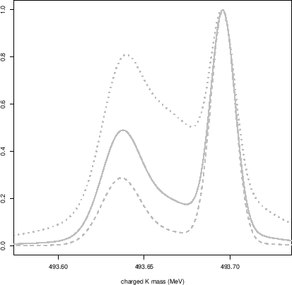
it is clear from the bottom plot of Fig. 10
that the results would be quite different.
,
the interpretation is tacitly Gaussian,
or it is assumed as such in further analyses [35].
For example, if one is
interested, for some deep physical reasons,
in the chance that the mass is
larger than 493.70 MeV,
it is clear from the bottom plot of Fig. 10
that the results would be quite different.
One might argue if, for such a
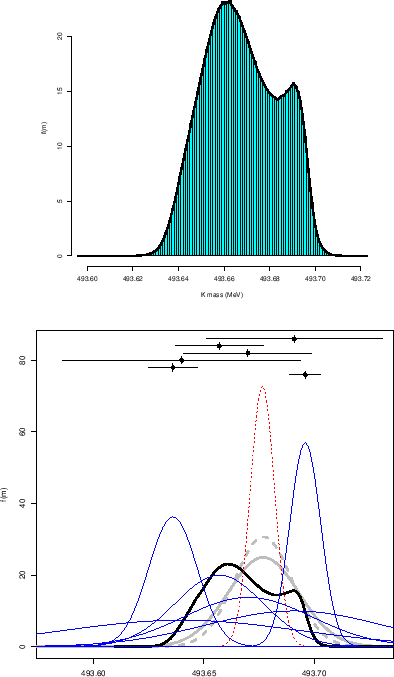
purpose, we could use the bi-modal curve of the PDG
ideogram (see Fig. 1),
in alternative to the pdf resulting from
the sceptical analysis performed here.
But what is the meaning of the bi-modal curve of Fig. 1?
If one compares it with the individual Gaussians reported
in Fig. 2 we see that it follows somehow
the profile of highest points of the curves. Therefore
the first guess is that it is just an unnormalized sum, that is
![]() . But
checking it, it does not seem to be the case. The second
guess was a kind of weighted average, with weights equal to
. But
checking it, it does not seem to be the case. The second
guess was a kind of weighted average, with weights equal to
![]() , i.e.
, i.e.
![]() ,
but it did not work either. The third attempt was to set the
weights to
,
but it did not work either. The third attempt was to set the
weights to ![]() , i.e.
, i.e.
![]() ,
and this seems to be the case.
The three attempts are reported in Fig. 11,
but just as a curiosity, as they have no probabilistic meaning.
,
and this seems to be the case.
The three attempts are reported in Fig. 11,
but just as a curiosity, as they have no probabilistic meaning.
 |
Let us end this section showing how to re-obtain
the standard combination with
the same general model used in the sceptical combination.
We just need to choose values
suitable ![]() and
and ![]() to get
to get
![]() and
and
![]() .
Inverting Eqs. (13) and (14) of [15] seems complicate,
but in the limit of zero variance, this is the same as requiring
.
Inverting Eqs. (13) and (14) of [15] seems complicate,
but in the limit of zero variance, this is the same as requiring
![]() and
and
![]() ,
a condition easier to apply in practice. Being in fact
,
a condition easier to apply in practice. Being in fact
![]() and
and
![]() ,
the requirement simply translates into
,
the requirement simply translates into
![]() with both parameters `very large'. In practice is is enough to set e.g.
with both parameters `very large'. In practice is is enough to set e.g.
![]() to recover the result of the weighed average
of
to recover the result of the weighed average
of
![]() MeV.
MeV.