Sceptical combination with `JAGS` - Preliminaries

It is now time to improve our model in order to implement what has been discussed in the introduction, where it was said that our skepticism would act on the variable $r_i = \sigma_i/s_i$ . However, following Ref. [16], in the previous paper on the subject [15] a different variable was indeed considered, namely $\omega_i = s_i^2/\sigma_i^2$ . The relations between the variables which enter the game are conveniently shown in the graphical model of Fig. 8, where the following convention has been used:

**Figure:** Graphical model behind the sceptical combination. The solid lines represent probabilistic links, the dashed ones deterministic links. The unusual dotted line stands for an auxiliary variable which is not really part of the model, but it is convenient to track.
$\begin{figure}\begin{center} \epsfig{file=skeptical_DL.epsi,clip=,} \end{center}\end{figure}$

arrows with solid lines represent - this is the usual convention - probabilistic links between parent(s) and child(ren), in our case depending from $\mu$ and $\tau_i$ ;
arrows with dashed lines represent deterministic links, that is $\tau_i = \omega_i/s_i^2$ ;
finally the arrow with dotted line is unusual, in the sense that it is not used in the literature. It is in fact still a deterministic link, being $r_i = 1/\sqrt{\omega_i}$ , but it is irrelevant for the model itself and it could be also (and perhaps better, as far as the efficiency of the program is concerned) calculated at the end of the sampling.

In the graphical model there are three kind parents having no `ancestors': $\mu$ , $\omega_i$ , and

. Therefore they need priors, that is $f(\mu\,\vert\,I)=f_0(\mu)$ , and so on. But

are simply constant and do not require priors (or, if you like, they are just Dirac delta's). For $f_0(\mu)$ we choose, as before, a practically flat prior obtained by a Gaussian distribution with very large $\sigma_0$ . The mathematically convenient prior of $\omega_i$ is instead a Gamma distribution, implying that the distribution of

is instead not an elementary one, as it can be seen comparing Eq. (11) and (12) of Ref. [15].

For the parameters of the Gamma pdf of $\omega_i$ we stick to those chosen in Ref. [15],¹⁸ i.e. $\delta=1.3$ and $\lambda=0.6$ , in order to get $\mbox{E}[r_i] = \sigma(r_i) = 1$ . Figure 9,

**Figure:** Examples of sceptical combinations taken from [15]. The plots on the left-hand side show the individual results. The plots on the right-hand side show the combined result obtained using a sceptical combination (continuous lines), compared with the standard combination (dashed lines).
$\begin{figure}\begin{center} \begin{tabular}{\vert c\vert c\vert}\hline Individ... ...eps,width=0.4\linewidth,clip=} \\ \hline \end{tabular}\end{center} \end{figure}$

taken from Fig. 4 of Ref. [15], shows how the model performs in some situations which represent kind of extreme cases with respect to the usual `disagreements' within a set of results.

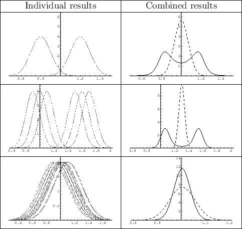Particularly interesting are the cases in which the individual results cluster in two regions, or when they overlap `too much'. In the first case, while the simple weighted average prefers mass values in a region where there is no experimental support, the sceptical combination exhibits a bimodal distribution, because we tend to believe with equal probability that the true value is in either side (but it could also be in the middle, although with low probability). In the second case, instead, in which the results overlap too much, the method has the nice feature of producing a pdf narrower than that obtained by the simple weighted average, reflecting our natural suspicion that the quoted uncertainties might have been overestimated. In Ref. [15] (Fig. 5 there) it was also studied how the results varied if the initial $\sigma(r_i)$ was allowed to move by $\pm 50\%$ . This leads us to be rather confident that the choice of $\delta=1.3$ and $\lambda=0.6$ is not critical.

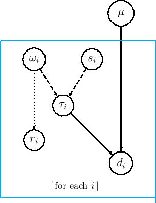
Here is, finally, the JAGS model, easy to understand if we compare it with the graphical model of Fig. 8:

var tau[N], r[N], omega[N];
model {
   for (i in 1:N) {
      d[i] ~ dnorm(mu, tau[i]);
      tau[i] <- omega[i]/s[i]^2;
      omega[i] ~ dgamma(delta, lambda);
      r[i] <- 1.0/sqrt(omega[i]);
   }
   mu  ~ dnorm(0.0, 1.0E-8);
}

Before running it, let us make a very trivial model in which JAGS is used as a simple random generator, without any inferential purpose, just to get confidence with the prior distribution of . Moreover, consisting the core of the model of just two lines of code, we write it directly from the R script into a temporary file. Here is the complete script, in which it also shown an alternative way (indeed the simplest one in R) to prepare the `list' data to be passed to JAGS via jags.model() - note the missing update(), because we deal here with direct sampling and there are no burn-in issues:

library(rjags)
data = list(delta=1.3, lambda=0.6)
model = "tmp_model.bug"
write("
model{
  omega ~ dgamma(delta, lambda);
  r <- 1.0/sqrt(omega);
}
", model)

jm <- jags.model(model, data)
chain <- coda.samples(jm, c("omega","r"), n.iter=10000)
plot(chain)
print(summary(chain))

This is the result of the last command:

1. Empirical mean and standard deviation for each variable,
   plus standard error of the mean:

        Mean     SD Naive SE Time-series SE
omega 2.1979 1.9127 0.019127       0.019065
r     0.9948 0.9096 0.009096       0.009096

2. Quantiles for each variable:

        2.5%    25%    50%   75% 97.5%
omega 0.1162 0.8045 1.6582 3.035 7.329
r     0.3694 0.5741 0.7766 1.115 2.934

We see that the (indirectly) sampled r has (with good approximation) the expected unitary mean and standard deviation. As a further check, let us use directly the Gamma random generator rgamma() of R,

r <- 1/sqrt(rgamma(10000, 1.3, 0.6))
cat(sprintf("mean(r) = %f, sd(r) = %f\n", mean(r), sd(r)))

whose (aleatory) result is left as exercise to the reader.

Sceptical combination with JAGS - Preliminaries

Sceptical combination with `JAGS` - Preliminaries