Implementation in JAGS/rjags

As a first example, here is the model to make the simple weighted average of the charged kaon mass values of Tab. 1 (we are indeed “breaking a nut with a mallet”):

model {
   for (i in 1:length(d)) {
      d[i] ~ dnorm(m, 1/s[i]^2);
   }
   m  ~ dnorm(0.0, 1.0E-8);
}

The loop is just the implementation of the graphical model on the right side of Fig. 5, with $x_i$ here called d[i] in order to maintain the notation used in Eqs. (1) and (2). dnorm() stands for normal distribution density function, whose parameters are the kaon mass m (equal for all measurements, because we believe they were measuring the same thing) and 1/s[i]ˆ2, that is $\tau_i$, as discussed in the previous subsection. The last line of code defines the prior of the mass value: formally a normal distribution, but in fact a flat one in the domain of interest, being $\sigma_0=10^4\,$MeV. The model is saved in the file weighted_average.bug and we move now to the R code.

First we assign the experimental values to the vector d and s (no declarations are required in R) and then we evaluate and print the weighed average and the combined standard deviation calculated from Eqs. (1) and (2):

d <- c(493.691, 493.657, 493.670, 493.640, 493.636, 493.696)
s <- c(  0.040,   0.020,   0.029,   0.054,   0.011,   0.007)
d.av  <- sum(d/s^2)/sum(1/s^2) 
s.av  <- 1/sqrt(sum(1/s^2))
cat(sprintf("combined value: %f +- %f\n", d.av, s.av))

Executing the script¹⁶containing these five lines, we get

combined value: 493.676599 +- 0.005478

that for the moment is just a check.

Let us now move to the rjags stuff in the R script:

library(rjags)   # load rjags 
data   <- NULL   # declare an empty list
data$d <- d      # first  element of the list
data$s <- s      # second element of the list
model  <- "weighted_average.bug"  

jm <- jags.model(model, data)                    # define the model
update(jm, 100)                                  # burn in 
chain <- coda.samples(jm, c("m"), n.iter=10000)  # sampling

So, first the package rjags is loaded calling the function library(), then we fill the data in the list¹⁷ data (arbitrary name) and we put the model file name into the string variable model (again arbitrary name). Finally we interact with JAGS in three steps:

1. the function jags.model(model, data) passes model and the data to JAGS; the model is compiled and, if everything is ok, a summary message is reported, like in this case

   Compiling model graph
      Resolving undeclared variables
      Allocating nodes
   Graph information:
      Observed stochastic nodes: 6
      Unobserved stochastic nodes: 1
      Total graph size: 29
   

2. then, update(jm, 100) lets the Markov chain do 100 moves in the parameter space, but without recording the values, so that the initial points are not taken into account when the chain if analyzed;
3. finally, coda.samples(jm, c("m"), n.iter=10000) does the real work, following the evolution of the chain for n.iter steps, the model variable m is monitored and the resulting history is returned and stored in the object chain (arbitrary name).

At this point JAGS has done its work and we only need to analyze its outcome. For this task the high level functions of R are very helpful. For example we can make a summary plot just calling plot(chain), whose result is shown in Fig. 7:

Figure: Summary plot of the chain returned by JAGS.

the left hand plot shows the history of m during the 10000 recorded iterations; the right hand one is a smoothed representation of the histogram of the sampled values of m.

R provides also a summary of the result, using the function summary(chain) $[$or, better, print(summary(chain)) if we want to include it into a script$]$, with many statistical informations like average, standard deviation and quantiles for each sampled variable. Or we can do it in more detail using the high level R functions. Here is, for example, how to calculate mean and standard deviation (also to show a way to extract the history of a single variable from the object returned by coda.samples()):

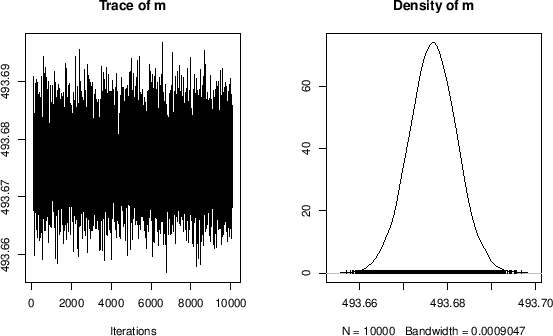
m.mean <- mean(chain[[1]][,'m'])
m.sd   <- sd(chain[[1]][,'m']) 
cat(sprintf("JAGS result: %f +- %f\n", m.mean, m.sd))

resulting (with this particular sampling) in

JAGS result: 493.676632 +- 0.005451

practically identical to the weighted average obtained using exact formulae.