Before we write down the model to solve our little problem
described by the graphical model of Fig. 5,
some words on the Gibbs sampling are needed, also to understand
why this kind
of programs do not use  as second parameter of the Gaussian,
but rather
as second parameter of the Gaussian,
but rather  , traditionally indicated by
  .
.
We have seen that if we have a problem with Gaussian error functions
and a flat prior on  , then
the posterior of is still a Gaussian, and it remains Gaussian
also if we assign to a Gaussian prior characterized by
, then
the posterior of is still a Gaussian, and it remains Gaussian
also if we assign to a Gaussian prior characterized by  and
and  , a flat prior being recovered
for
, a flat prior being recovered
for
 (and allow me to draw again your
attention on footnote 9).
Let us see what happens if we are also in condition
of uncertainty concerning ,
assumed to be the same in all
(and allow me to draw again your
attention on footnote 9).
Let us see what happens if we are also in condition
of uncertainty concerning ,
assumed to be the same in all  measurements (typical problem
of when we collect a sample a measurements under apparently
the same conditions and we are interested in inferring
both and ). The graphical model
is still the one on the right hand side of Fig. 5,
but with
measurements (typical problem
of when we collect a sample a measurements under apparently
the same conditions and we are interested in inferring
both and ). The graphical model
is still the one on the right hand side of Fig. 5,
but with
 for all
  .
The analogue of Eq. (3) is now
.
The analogue of Eq. (3) is now
Applying the chain rule only to  and
and  ,
to begin,
and noting that and do not depend on each other,
as it is usually the case,13we have, instead of Eq. (4),
,
to begin,
and noting that and do not depend on each other,
as it is usually the case,13we have, instead of Eq. (4),
Equations
(5) becomes then, also extending Eq. (15)
to all  ,
,
Now, if for some reasons we fix to the
hypothetical value  (and for simplicity we use a flat
prior for ) then we recover, without any calculation,
something similar to Eq. (12):
(and for simplicity we use a flat
prior for ) then we recover, without any calculation,
something similar to Eq. (12):
where now  is simply the arithmetic average
and
is simply the arithmetic average
and
 . If we had taken into account
a prior
. If we had taken into account
a prior  modeled by a Gaussian, then
 would still be a Gaussian, as we have seen above.
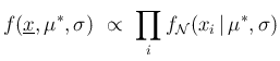
In particular, it easy to sample by
Monte Carlo the
`random' variable described by Eq. (16),
because it is rather easy to write a
Gaussian `random' number generator, or to use one of those available
in the mathematical libraries of programming languages.
would still be a Gaussian, as we have seen above.
In particular, it easy to sample by
Monte Carlo the
`random' variable described by Eq. (16),
because it is rather easy to write a
Gaussian `random' number generator, or to use one of those available
in the mathematical libraries of programming languages.
Let us now do the opposite exercise, the utility
of which will be clear in a while: imagine we are interested
in
 ,
having imposed the condition
,
having imposed the condition  .
Equations (6) and
(7) are now turned into
(note the factor
.
Equations (6) and
(7) are now turned into
(note the factor  in front of each exponent,
since it cannot be any longer absorbed in the normalization constant!)
in front of each exponent,
since it cannot be any longer absorbed in the normalization constant!)
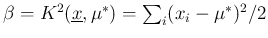
where
 is a constant, given
  and
and  , written in a way to remind that it is
by definition non negative. Unfortunately, opposite to the case
of
, written in a way to remind that it is
by definition non negative. Unfortunately, opposite to the case
of
 , this is an unusual form
in probability theory. But a simple change of variable
rescues us. In fact, if instead of we use
, this is an unusual form
in probability theory. But a simple change of variable
rescues us. In fact, if instead of we use
 ,
then the last equation becomes
,
then the last equation becomes
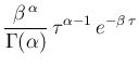
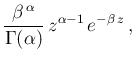
in which probability and statistics experts recognize
a Gamma distribution, usually written for the generic variable  as
as
where  is the Gamma function
(and hence the name of the distribution).
Therefore
is the Gamma function
(and hence the name of the distribution).
Therefore
with
 and
and
 .
Being this a well known probability distribution,
there are formulae available for the summaries
of interest.14For example, expected value and variance
are given by
.
Being this a well known probability distribution,
there are formulae available for the summaries
of interest.14For example, expected value and variance
are given by  and
and
 , respectively.
But, moreover, there are Gamma random generators available, which
is what we need for sampling.
, respectively.
But, moreover, there are Gamma random generators available, which
is what we need for sampling.
We are then finally ready to describe the Gibbs sampler algorithm,
applied to our two-dimensional case
(but it can be applied in higher dimensionality problems too):
- start choosing an arbitrary initial point
 in the
  plane;
- extract `at random' a new value of , let it be
 ,
given
,
given  , from
 ;
;
- extract then `at random' a new value of , let it be
 ,
given , from
,
given , from
 ;
;
- extract then `at random' a new value of , let it be
 ,
from
,
from
 ;
;
- continue on, through the steps
 .
.
(And, obviously, for each  there is a related
  .)
Now, amazing enough (but there are mathematical
theorems ensuring the `correct' behavior [21]),
the points so obtained sample the bi-dimensional
distribution , and then
.)
Now, amazing enough (but there are mathematical
theorems ensuring the `correct' behavior [21]),
the points so obtained sample the bi-dimensional
distribution , and then  , in the sense that
the expected frequency to visit a given region is proportional
to the probability of that region (just Bernoulli theorem,
not to be confused with the frequentist `definition' of
probability! - see e.g. Ref. [31]).
Moreover, for the way it has been described, it is clear that the probability
of the move
, in the sense that
the expected frequency to visit a given region is proportional
to the probability of that region (just Bernoulli theorem,
not to be confused with the frequentist `definition' of
probability! - see e.g. Ref. [31]).
Moreover, for the way it has been described, it is clear that the probability
of the move
 depends
only
depends
only
 and not on the previous states.
This is what defines a Markov Chain Monte Carlo, of which the
Gibbs sample is one of the possible algorithms.
and not on the previous states.
This is what defines a Markov Chain Monte Carlo, of which the
Gibbs sample is one of the possible algorithms.
There is still the question of  , less trivial
then , because has to be
positive.15In this case a convenient prior would be a Gamma, with
, less trivial
then , because has to be
positive.15In this case a convenient prior would be a Gamma, with
 and
and  properly chosen, because
it easy to see that, when multiplied by
Eq. (19), the result is still a Gamma:
properly chosen, because
it easy to see that, when multiplied by
Eq. (19), the result is still a Gamma:
We can easily see that a flat prior for
is recovered in the limit
 and
and
 .
.
A last comment concerning the initial point for the sampling
is in order.
Obviously, the initial steps of the history (the sequence)
depend on our choice, and therefore they can be somehow
not `representative'. The usual procedure to overcome
this problem consists in discarding
the `first points' of the sequence, better if after
a visual inspection, or using criteria based on past experience
(notoriously, this kind of techniques are between science and art,
even when they are grounded on mathematical theorems, which
however only speak of `asymptotic behavior').
But, as a matter of fact, the convergence of the Gibbs sampler
for low dimensional problems is very fast and modern computers
are so powerful that, in the case of doubt,
we can simply throw away several thousands initial
points `just for security'.
![\begin{eqnarray*}
f(\underline{x},\mu,\sigma\,\vert\,I) & = &
\left[ \prod_i f...
...mu,\sigma)\right]\cdot
f_0(\mu)\cdot f_0(\sigma) \,. \nonumber
\end{eqnarray*}](img125.png)
![$\displaystyle \frac{1}{\sqrt{2\,\pi}\,\sigma_C}\, \exp\left[- \frac { (\mu-\overline{x})^2}
{2\,\sigma_C^2} \right]$](img106.png)
![$\displaystyle \prod_i\,
\frac{1}{\mathbf{\sigma}}\,
\exp\left[-\frac{(x_i-\mu^*)^2}{2\,\sigma^2}\right]$](img135.png)
![$\displaystyle \frac{1}{\mathbf{\sigma}^n}\,
\exp\left[-\frac{\sum_i(x_i-\mu^*)^2}{2\,\sigma^2}\right]$](img136.png)
![$\displaystyle \frac{1}{\mathbf{\sigma}^n}\,
\exp\left[-\frac{K^2(\underline{x},\mu^*)}{\sigma^2}\right] \,,$](img137.png)