Model and analysis method

Dealing with problems of this kind, we have learned (see e.g. [17]) the importance of building up a graphical representation of the causal model relating the quantities of interest, some of them `observed' and others `unobserved', among the latter the quantities we wish to infer. Also in this case, despite some initial skepticism about the possibility of getting some meaningful results, once we have built up the model, very basic indeed, it was clear that the main outcome concerning the vaccine efficacy was not depending on the many aspects of the trials. Our initial doubts were in fact related to the several details concerning the people involved in the test campaign, but they finally resulted to be much less critical than we had at first thought.

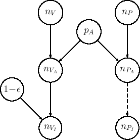
The causal model used in this analysis is implemented in the Bayesian network of Fig. .

**Figure:** *Simplified Bayesian network of the vaccine vs placebo experiment (see text).*
$\begin{figure}\begin{center} \epsfig{file=vaccine_eff.eps,clip=,width=0.5\linewidth} \\ \mbox{} \vspace{-1.0cm} \mbox{} \end{center} \end{figure}$

The top nodes

and

stand for the number of individuals in the vaccine and placebo (i.e. control) groups, respectively, as the subscripts indicate, while the bottom ones ( $n_{V_I}$ and $n_{P_I}$ ) are the number of individuals of the two groups resulting infected during the trial. These are the observed nodes of our model and their values are summarized in Tab.

Then, there is the question of how to relate the numbers of infectees to the numbers of the participants in the trial. This depends in fact on several variables, like the prevalence of the virus in the population(s) of the involved people, their social behavior, personal life-style, age, health state and so on. And, hopefully, it depends on the fact that a person has been vaccinated or not. Lacking detailed information, we simplify the model introducing an assault probability , that is a catch-all term embedding the many real life variables, apart being vaccinated or not. Nodes $n_{V_A}$ and $n_{P_A}$ in the network of Fig. represent then the number of `assaulted individuals' in each group, and they are modeled according to binomial distributions, that is

$\displaystyle n_{V_A}$	$\displaystyle \sim$	Binom $\displaystyle (n_V, p_A)$	(1)
$\displaystyle n_{P_A}$	$\displaystyle \sim$	Binom $\displaystyle (n_P, p_A)\,,$	(2)

represented in the graphical model by solid arrows.

The `assaulted individuals' of the control group are then assumed to be all infected, and hence the deterministic link with dashed arrow relating node $n_{P_A}$ to node $n_{P_I}$ follows (indeed the two numbers are exactly the same in our model, and we make this distinction only for graphical symmetry with respect to the vaccine group).

Instead, the `assaulted individuals' of the other group are `shielded' by the vaccine with probability $\epsilon$ , that we therefore identify with efficacy, although we shall come back at the due point about what should be reported as `efficacy'. The probability of becoming infected if assaulted is therefore equal to $1\!-\!\epsilon$ , so that node $n_{V_I}$ is related to node $n_{V_A}$ by

$\displaystyle n_{V_I}$

$\displaystyle \sim$

Binom $\displaystyle (n_{V_A}, 1\!-\!\epsilon).$

(3)

At this point all the rest is a matter of calculations, that we do by MCMC techniques⁴with the help of the program JAGS [15] interfaced with R [18] via rjags [19].

The nice thing using such a tool is that we have to take care only to describe the model, with instructions whose meaning is quite transparent:⁵

      model {
        nP.I  ~ dbin(pA, nP)           # 1.          
        nV.A  ~ dbin(pA, nV)           # 2.
        pA    ~ dbeta(1,1)             # 3. 
        nV.I  ~ dbin(ffe, nV.A)        # 4.  [ ffe = 1 - eff ]
        ffe   ~ dbeta(1,1)             # 5.
        eff   <- 1 - ffe               # 6. 
      }

We easily recognize in lines 1. and 2. of the R code the above Eqs. (

) and (

), while line 4. stands for Eq. (

). Line 6. is simply the transformation of ` $1\!-\!\epsilon$ ' (`ffe' in the code) to $\epsilon$ , the quantity we want to trace in the `chain'. Finally lines 3. and 5. describe the priors of the `unobserved nodes' that have no `parents', in this case

and $1\!-\!\epsilon$ . We use for both a uniform prior, modeled by a Beta distribution (see Sec.

for details) with parameters $\{1,\,1\}$ .⁶ Then we have to provide the data, in our case

, $n_{V_I}$ and $n_{P_I}$ . The program samples the space of possibilities and returns lists of numbers (a `chain') for each `monitored variable', which can then be analyzed `statistically'. For example the frequency of occurrence of the values in each list is expected to be proportional to the probability of that values of the variable (Bernoulli's theorem). Similarly we can evaluate correlations among variables.

Table: Top table: MCMC results for the model parameter $\epsilon$ (see text). Bottom table: same as Tab. for easier comparison with the MCMC results.

MCMC results

	mean $\pm$ stand. unc.	centr. 95% cred. int.	$P(\epsilon \ge 0.9)$
Moderna-1	$0.933 \pm 0.028$		0.875
Moderna-2	$0.935 \pm 0.019$		0.951
Pfizer	$0.944 \pm 0.019$		0.974
AstraZeneca LDSD	$0.861 \pm 0.075$		0.349
AstraZeneca SDSD	$0.599 \pm 0.090$		0.000

Published results

	efficacy value	95% `uncertainty interval'
Moderna-1 [5]		-----
Moderna-2 [7]		(confidence interval)
Pfizer [4]		(credible interval)
AstraZeneca LDSD [8]		(confidence interval)
AstraZeneca SDSD [8]		(confidence interval)