Model and analysis method

The causal model used is represented in the Bayesian network of Fig. 1.

Figure: Simplified Bayesian network of the vaccine vs placebo experiment (see text).

The top nodes $n_V$ and $n_P$ stand, respectively, for the number of individual in the vaccine and placebo groups, as the subscripts indicate, while the bottom ones ($n_{V_I}$ and $n_{P_I}$) are the number of individuals of the two groups resulting infected after the trial period.

The sure data are $n_{V_I}=5$ and $n_{P_I}=90$ for Moderna [2] and $n_{V_I}=8$ and $n_{P_I}=162$ for Pfizer [6]. As far as the number of individual subject to the trials there were certainly some information in the press releases, but, fortunately, as we shall see, the exact number is not critical at all in regard to the value of efficacy and we can even change it by orders of magnitudes without affecting the results of interest.

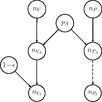
Then, there was the question of how to relate the numbers of infected to the numbers of the participants in the trial. This depends in fact from several variables, like the prevalence of the virus in the population(s) of the involved people, their life-style, behavior, and so on, and, hopefully, from the fact that a person has been vaccinated or not. We simplified the model defining an assault probability, $p_A$, a catch-all term embedding the many real life variables, apart being vaccinated or not. Nodes $n_{V_A}$ and $n_{P_A}$ represent them the number of `assaulted individuals' in each group, and they are modeled according to a binomials distributions, that is

$$n_{V_A} \sim (n_V, p_A)$$ (1)

$$n_{P_A} \sim (n_P, p_A)\,,$$ (2)

represented in the graphical model by solid arrows.

The `assaulted individuals' of the placebo group are then assumed to be all infected, and hence the deterministic link with dashed arrow relating the node $n_{P_A}$ to the node $n_{P_I}$ (in fact the two numbers are the same, and we make this graphical distinction only for symmetry with respect to the vaccine group).

Instead, the `assaulted individuals' of the other group are `shielded' by the vaccine, with probability of being infected equal to $1\,-\,\epsilon$, where $\epsilon$ is the efficacy:

$$n_{V_I} \sim (n_{V_A}, 1\!-\!\epsilon).$$ (3)

At this point all the rest is a matter of calculations, that we do by Markov Chain Monte Carlo (MCMC) techniques with the help of the program JAGS [7] interfaced with R [8] via rjags [9].

The nice thing using such a tool is that we have to take care only to describe the model, with instructions whose meaning is rather transparent. Then we have to provide the data, in our case $n_V$, $n_P$, $n_{V_I}$ and $n_{P_I}$. The program samples the space of possibilities and returns lists of numbers (a `chain') for each `monitored variable' such that the frequency of the values in each list is proportional to the probability of that values of the variable (Bernoulli's theorem). Here is, verbatim, the model:

      model {
        nP.I  ~ dbin(pA, nP)           # 1.          
        nV.A  ~ dbin(pA, nV)           # 2.
        pA    ~ dbeta(1,1)             # 3. 
        nV.I  ~ dbin(ffe, nV.A)        # 4.  [ ffe = 1 - eff ]
        ffe   ~ dbeta(1,1)             # 5.
        eff   <- 1 - ffe               # 6. 
      }

We easily recognize in lines 1. and 2. of the code Eqs. (1) and (2), while line 4. stands for Eq. (3). Line 6. is simply the transformation of ` $1\!-\!\epsilon$' (`ffe' in the code) to $\epsilon$, the quantity we want to trace in the chain. Finally lines 3. and 5. describe the priors of the `unobserved nodes' that have no `parents', in this case $p_A$ and $1\!-\!\epsilon$. We use in both cases a uniform prior, modeled by a Beta distributions with both parameters equal to 1 (we cannot go into the details of this choice that we consider quite reasonable, given the information provided by the data, and refer for the details to Ref. [5] and references therein). Finally, those who have no experience with JAGS can find in Ref. [5] several ready-to-run R scripts.