Some rules of thumb to unfold probabilistic sensible information from results published with asymmetric uncertainties

Having understood what one should have done to obtain expected value and standard deviation in the situations in which people are used to report asymmetric uncertainties, we might attempt to recover those quantities from the published result. It is possible to do it exactly only if we know the detailed contributions to the uncertainty, namely the $\chi ^2$ or log-likelihood functions of the so called `statistical terms' and the pairs $\{\Delta_{+_i}, \Delta_{-_i}\}$, together to the probabilistic model, for each `systematic term'. However, these pieces of information are usually unavailable. But we can still make some guesses, based on some rough assumptions, lacking other information:

• asymmetric uncertainties in the `statistical part' are due to asymmetric $\chi ^2$ or log-likelihood: $\rightarrow$ apply corrections given by Eqs. (15)-(16);
• asymmetric uncertainties in the `systematic part' comes from nonlinear propagation: $\rightarrow$ apply corrections given by Eqs. (28)-(29).

As a numerical example, imagine we read the following result (in arbitrary units):

$$Y = 6.0 ^{+1.0}_{-2.0} ^{+0.3}_{-0.9} ,$$ (30)

(that somebody would summary as $6.0 ^{+1.0}_{-2.2}$!). The only certainty we have, seeing two asymmetric uncertainties with the same sign of skewness, is that the result is definitively biased. Let us try to make our estimate of the bias and calculate the corrected result (that, not withstanding all uncertainties about uncertainties, will be closer to the `truth' than the published one):

1. the first contribution gives roughly [see. Eqs. (15)-(16)]:
   

   $$\delta_1 \approx -1.0$$ (31)

   $$\sigma_1 \approx 1.5 ;$$ (32)

   
   

2. for the second contribution we have [see. Eqs. (24)-(24), (28)-(29)]:
   

   $$\delta_2 \approx -0.31$$ (33)

   $$\sigma_2 \approx 0.62 .$$ (34)

   
   

Our guessed best result would then become¹⁴

$$Y \approx 4.69 \pm 1.5 \pm 0.62 = 4.69 \pm 1.62$$ (35)

$$\approx 4.7 \pm 1.6 .$$ (36)

(The exceeding number of digits in the intermediate steps are just to make numerical comparison with the correct result that will be given in a while.)

If we had the chance to learn that the result of Eq. (30) was due to the asymmetric $\chi ^2$ fit of Fig. 2 plus two systematic corrections, each described by the triangular distribution of Fig. 1, then we could calculate expectation and variance exactly:

$$\mbox{E}(Y) = 4.2 + 2\times 0.17 = 4.54$$ (37)

$$\sigma^2(Y) = 1.5^2 + 2\times 0.42^2 = 1.61^2 ,$$ (38)

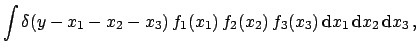
i.e. $Y=4.54\pm 1.61$, quite different from Eq. (30) and close to the result corrected by rule of thumb formulae. Indeed, knowing exactly the ingredients, we can evaluate $f(y)$ from Eq.(1) as

$$f(y) = \int \delta(y - x_1 - x_2 - x_3) f_1(x_1) f_2(x_2) f_3(x_3) \mbox{d}x_1 \mbox{d}x_2 \mbox{d}x_3 ,$$ (39)

although by Monte Carlo.

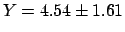
Figure: Monte Carlo estimate of the shape of the p.d.f. of the sum of three independent variables, one described by the p.d.f. of Fig. 2 and the other two by the triangular distribution of Fig. 1.

The result is given in Fig. 5, from which we can evaluate a mean value of 4.54 and a standard deviation of 1.65 in perfect agreement with the figures given in Eqs. (37)-(38).¹⁵ As we can see from the figure, also those who like to think at 'best value' in term of most probable value have to realize once more that the most probable value of a sum is not necessarily equal to the sum of most probable values of the addends (and analogous statements for all combinations of uncertainties¹⁶). In the distribution of Fig. 5, the mode of the distribution is around 5. [Note that expected value and variance are equal to those given by Eqs. (37)-(38, since in the case of a linear combination they can be obtained exactly.] Other statistical quantities that can be extracted by the distribution are the median, equal to 4.67, and some 'quantiles' (values at which the cumulative distribution reaches a given percent of the maximum - the median being the 50% quantile). Interesting quantiles are the 15.85%, 25%, 75% and 84.15%, for which the Monte Carlo gives the following values of $Y$: 2.88, 3.49, 5.72 and 6.18. From these values we can calculate the central 50% and 68.3% intervals,¹⁷which are $[3.49, 5.72]$ and $[2.88, 6.18]$, respectively. Again, the information provided by Eq. (30) is far from any reasonable way to provide the uncertainty about $Y$, given the information on each component.

Besides the lucky case¹⁸of this numerical example (which was not constructed on purpose, but just recycling some material from Ref. [3]), it seems reasonable that even results roughly corrected by rule of thumb formulae are already better than those published directly with asymmetric result.¹⁹ But the accurate analysis can only be done by the authors who know the details of the individual contribution to the uncertainty.