Next: Uncertainty on the expected
Up: Inferring the success parameter
Previous: Meaning and role of
Poisson background on the observed number of
`successes'
Imagine now that the  successes might contains an unknown number
of background events
successes might contains an unknown number
of background events  , of which we only know their
expected value
, of which we only know their
expected value  , estimated somehow and
about which we are quite sure (i.e. uncertainty about
is initially neglected -- it will be indicated at the end
of the section how to handle it).
We make the assumption that the background events
come at random and are described by a Poisson process of
intensity
, estimated somehow and
about which we are quite sure (i.e. uncertainty about
is initially neglected -- it will be indicated at the end
of the section how to handle it).
We make the assumption that the background events
come at random and are described by a Poisson process of
intensity  , such that the Poisson parameter
is equal to
, such that the Poisson parameter
is equal to
 in the domain of time, with
  the
observation time. (But we could as well reason in
other domains, like objects per unit of length, surface,
volume, or solid angle. The density/intensity parameter
the
observation time. (But we could as well reason in
other domains, like objects per unit of length, surface,
volume, or solid angle. The density/intensity parameter  will have different dimensions depending on the context, while
 will always be dimensionless.)
The number of observed successes has now two contributions:
In order to use Bayes theorem we need to calculate
 , that is
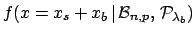 ,
i.e. is the probability function of the sum
of a binomial variable and a Poisson variable.
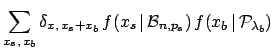
The combined probability function is give by (see e.g. section 4.4
of Ref. [2]):
,
i.e. is the probability function of the sum
of a binomial variable and a Poisson variable.
The combined probability function is give by (see e.g. section 4.4
of Ref. [2]):
where
 is the Kronecker delta that constrains
the possible values of
is the Kronecker delta that constrains
the possible values of
 and in the sum ( and run from 0 to
the maximum allowed by the constrain).
Note that we do not need to
calculate this probability function for all , but only
for the number of actually observed successes.
and in the sum ( and run from 0 to
the maximum allowed by the constrain).
Note that we do not need to
calculate this probability function for all , but only
for the number of actually observed successes.
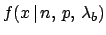
The inferential result about  is finally given by
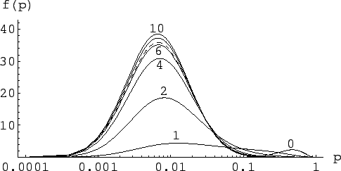
An example is shown in Fig. 5, for  ,
,  and an
expected number of background events
ranging between 0 and 10, as described in the
figure caption.
and an
expected number of background events
ranging between 0 and 10, as described in the
figure caption.
Figure:
Inference of for , ,
and several hypotheses of background
(right to left curves for
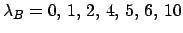 )
and two different priors (dashed lines),
)
and two different priors (dashed lines),
 in the upper plot and
 in the lower plot
(see text).
in the lower plot
(see text).
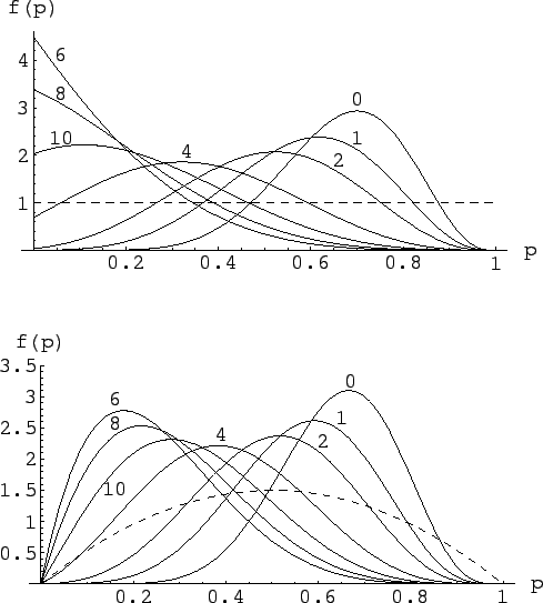 |
The upper plot of the figure is obtained by a uniform prior
(priors are represented with dashed lines in this figure).
As an exercise, let us also show in the lower plot of the figure
the results obtained using a broad prior still centered
at  , but that excludes the extreme values 0 and 1,
as it is often the case in practical cases.
This kind of prior has been modeled here with a beta function
of parameters
, but that excludes the extreme values 0 and 1,
as it is often the case in practical cases.
This kind of prior has been modeled here with a beta function
of parameters  and
and  .
.
For the cases of expected background different from zero
we have also evaluated
the  function, defined in
analogy to Eq. (27) as
function, defined in
analogy to Eq. (27) as
 Note that, while Eq. (27) is only defined
for
Note that, while Eq. (27) is only defined
for  , since a single observation makes
  impossible,
that limitation does not hold any longer
in the case of not null expected background.
In fact, it is important
to remember that, as soon as we have background,
there is some chance
that all observed events are due to it
(remember that a Poisson variable is defined for all non negative
integers!).
This is essentially the reasons why in this case the
likelihoods tend to a positive value for
impossible,
that limitation does not hold any longer
in the case of not null expected background.
In fact, it is important
to remember that, as soon as we have background,
there is some chance
that all observed events are due to it
(remember that a Poisson variable is defined for all non negative
integers!).
This is essentially the reasons why in this case the
likelihoods tend to a positive value for
 (I like to call `open' this kind of likelihoods [2]).
Figure:
Relative believe updating factor
of for , and
several hypotheses of background:
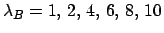 .
.
 |
As discussed above, the power of the data to update the believes on
is self-evident in a log-plot. We seen in Fig. 6 that,
essentially, the data do not provide any
relevant information for values of below 0.01.
Let us also see what happens when the prior concentrates our beliefs at small
values of , though in principle allowing all values of from 0 to 1.
Such a prior can be modeled with a log-normal distribution of suitable
parameters (-4 and 1), i.e.
![$f_0(p) = \exp\left[-(\log{p}+4)^2)/2\right]/(\sqrt{2\,\pi}\,p)$](img166.png) ,
with an upper cut-off at
,
with an upper cut-off at  (the probability that such
a distribution gives a value above 1 is
(the probability that such
a distribution gives a value above 1 is  ).
Expected value and standard deviation of Lognormal(-4,1) are
0.03 and 0.04, respectively.
).
Expected value and standard deviation of Lognormal(-4,1) are
0.03 and 0.04, respectively.
Figure:
Inference of for , ,
assuming a log-normal prior (dashed line) peaked at low , and with
several hypotheses of background
(
 ).
).
 |
The result is given in Fig. 7,
where the prior is indicated with a dashed line.
We see that, with increasing expected background, the posteriors are
essentially equal to the prior. Instead, in case of null background,
ten trials are already sufficiently to dramatically change our prior
beliefs. For example, initially there was 4.5% probability
that was above 0.1. Finally there is only 0.09% probability
for to be below 0.1.
The case of null background is also shown in
Fig. 8, where the results of the
three different priors are compared.
Figure:
Inference of for , in absence of background,
with three different priors.
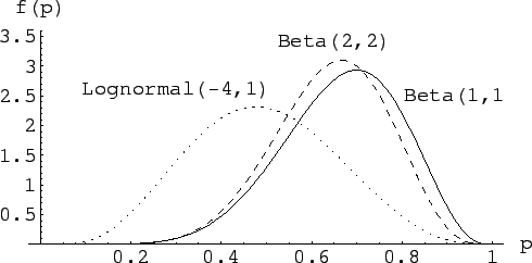 |
We see that passing from a
to a
,
makes little change in the conclusion. Instead, a log-normal prior
distribution peaked at low values of changes quite a lot the shape
of the distribution, but not really the substance of the result
(expected value and standard deviation
for the three cases are: 0.67, 0.13; 0.64, 0.12; 0.49, 0.16).
Anyway, the prior does correctly its job and there should be
no wonder that the final pdf drifts somehow to the left side,
to take into account a prior knowledge according to
which 7 successes in
10 trials was really a `surprising event'.
Those who share such a prior need more solid data to be convinced that
could be much larger than what they initially believed.
Let make the exercise of looking at what happens if a second
experiment gives exactly the same outcome ( with ).
The Bayes formula is applied sequentially, i.e. the posterior
of the first inference become the prior of the second inference.
That is equivalent to multiply the two priors (we assume
conditional independence of the two observations).
The results are given in Fig. 9.
Figure:
Sequential inference of
, starting from a prior peaked at low values,
given two experiments, each with and .
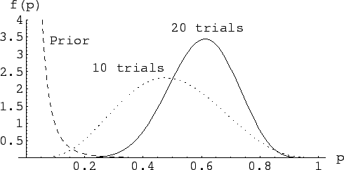 |
(By the way, the final result is equivalent to having observed
14 successes in 20 trials, as it should be -- the correct updating
property is one of the intrinsic nice features of the Bayesian approach).
Subsections
Next: Uncertainty on the expected
Up: Inferring the success parameter
Previous: Meaning and role of
Giulio D'Agostini
2004-12-13