


Next: Propagazioni di incertezza, approssimazioni
Up: Effetti sistematici e di
Previous: Effetti sistematici e di
Indice
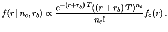 |
(14.1) |
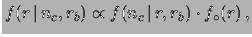
and, making use of Bayes' theorem, we get
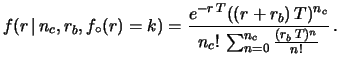 |
(14.2) |
 |
(14.3) |
- A uniform distribution between 0 and 30:
 |
(14.4) |
- A triangular distribution:
 |
(14.5) |
- A half-Gaussian distribution of
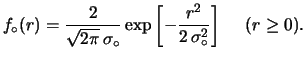
![$\displaystyle f_\circ(r) = \frac{2}{\sqrt{2\pi}\,\sigma_\circ} \exp\left[-\frac{r^2}{2\,\sigma_\circ^2}\right] \hspace{0.5cm}(r \ge 0).$](img3682.png) |
(14.6) |
Figura:
The upper plot shows some
reasonable priors reflecting the positive
attitude of researchers: uniform distribution (continuous);
triangular distribution (dashed); half-Gaussian distribution (dotted).
The lower plot shows how the results of
Fig. ![[*]](file:/usr/lib/latex2html/icons/crossref.png) , obtained
starting from an improper uniform distribution,
(do not) change if, instead, the
priors of the upper plot are used.
, obtained
starting from an improper uniform distribution,
(do not) change if, instead, the
priors of the upper plot are used.
 |
 |
(14.7) |
and consider only two possible values of  , let them be
  and
and 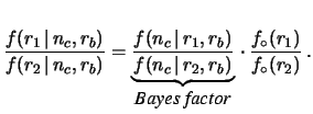 .
From (14.7) it follows that
.
From (14.7) it follows that
 |
(14.8) |
The Bayes factor can be extended to a continuous set of hypotheses ,
considering a function which gives the Bayes factor
of each value of with respect to a reference value  .
The reference value could be arbitrary, but for our problem the choice
.
The reference value could be arbitrary, but for our problem the choice
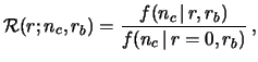 , giving
 |
(14.9) |
is very convenient for comparing and combining
the experimental results [#!ci!#,#!zeus!#,#!higgs!#].
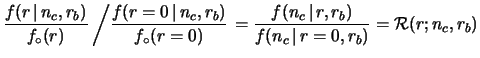
The function  has nice
intuitive interpretations which can be highlighted by
reordering the terms of (14.8) in the form
has nice
intuitive interpretations which can be highlighted by
reordering the terms of (14.8) in the form
 |
(14.10) |
(valid for all possible a priori values).
has the probabilistic interpretation of relative belief
updating ratio, or the geometrical interpretation
of shape distortion function of the probability density function.
goes to 1 for
 , i.e. in the asymptotic region
in which the experimental sensitivity is lost: As long as it is 1,
the shape of the p.d.f. (and therefore the relative probabilities in that
region) remains unchanged. Instead, in the limit
, i.e. in the asymptotic region
in which the experimental sensitivity is lost: As long as it is 1,
the shape of the p.d.f. (and therefore the relative probabilities in that
region) remains unchanged. Instead, in the limit
 (for large )
the final p.d.f. vanishes, i.e. the beliefs go
to zero no matter how strong they were before.
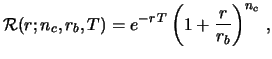
In the case of the Poisson process we are considering, the relative
belief updating factor becomes
(for large )
the final p.d.f. vanishes, i.e. the beliefs go
to zero no matter how strong they were before.
In the case of the Poisson process we are considering, the relative
belief updating factor becomes
 |
(14.11) |
with the condition14.1 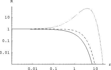 if
if  .
.
Figura:
Relative belief updating ratio
for the Poisson intensity parameter for the cases
of Fig. .
 |
These curves transmit the result of the experiment
immediately and intuitively:
- whatever one's beliefs on were before the data, these curves
show how one must14.2 change them;
- the beliefs one had
for rates far above 20 events/month are killed by the
experimental result;
- if one believed strongly that the rate had to be below
0.1 events/month, the data are irrelevant;
- the case in which no candidate events
have been observed gives the strongest constraint on the
rate ;
- the case of five candidate events over an expected background of
one produces a
peak of which corroborates the beliefs
around 4 events/month only if there were sizable
prior beliefs in that region.
Moreover there are some technical advantages in reporting
the function as a result of a search experiment.
- One deals with numerical values which can differ from unity
only by a few orders of magnitude in the region of interest,
while the values of the likelihood can be extremely low.
For this reason, the comparison between different
results given by the function can be perceived
better than if these results were published in terms of likelihood.
- Since differs from the likelihood only
by a factor, it can be used directly in Bayes' theorem,
which does not depend on constants, whenever
probabilistic considerations are needed.14.3In fact,
 |
(14.12) |
- The combination of different independent
results on the same14.4
quantity
can be done straightforwardly by multiplying individual
functions:
- Finally, one does not need to decide a priori if one wants to make a
`discovery' or an `upper limit' analysis as
conventional statistics teaches (see e.g. criticisms in
Ref. [#!BB!#]):
the function
represents the most unbiased way of presenting the results
and everyone can draw their own conclusions.
Next: Propagazioni di incertezza, approssimazioni
Up: Effetti sistematici e di
Previous: Effetti sistematici e di
Indice
Giulio D'Agostini
2001-04-02