Next: Other comments, examples and
Up: Bayesian unfolding
Previous: Bayes' theorem stated in
Contents
If one observes 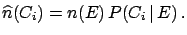 events with effect
  , the expected
number of events assignable to each of the causes is
, the expected
number of events assignable to each of the causes is
 |
|
|
(7.2) |
As the outcome of a measurement one has several possible effects
 (
(
 ) for a given cause
 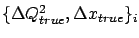 .
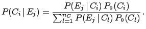
For each of them the
Bayes formula
(
.
For each of them the
Bayes formula
(![[*]](file:/usr/lib/latex2html/icons/crossref.png) )
holds, and
)
holds, and
 can be evaluated.
Let us write ()
again in the case of
can be evaluated.
Let us write ()
again in the case of  possible effects7.1,
indicating the initial probability of the causes with
possible effects7.1,
indicating the initial probability of the causes with
 :
:
 |
(7.3) |
One should note the following.
-
 , as usual.
Note that if the probability of a cause
is initially set to zero it can never change, i.e. if a cause
does not exist it cannot be invented.
, as usual.
Note that if the probability of a cause
is initially set to zero it can never change, i.e. if a cause
does not exist it cannot be invented.
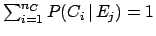
-
 .
This normalization condition, mathematically
trivial since it comes directly from (),
indicates that
each effect must come from one or more of the
causes under examination. This means that if the
observables also contain
a non-negligible amount of background, this needs to be included
among the causes.
.
This normalization condition, mathematically
trivial since it comes directly from (),
indicates that
each effect must come from one or more of the
causes under examination. This means that if the
observables also contain
a non-negligible amount of background, this needs to be included
among the causes.
-
 .
There is no need for
each cause to produce at least
one of the effects.
.
There is no need for
each cause to produce at least
one of the effects.
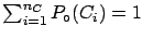
 gives the efficiency of finding the
cause in any of the possible effects.
gives the efficiency of finding the
cause in any of the possible effects.
After  experimental observations one obtains
a distribution of frequencies
experimental observations one obtains
a distribution of frequencies

 .
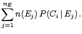
The expected number of events
to be assigned
to each of the causes (taking into account only the observed events)
can be calculated by applying () to each effect:
.
The expected number of events
to be assigned
to each of the causes (taking into account only the observed events)
can be calculated by applying () to each effect:
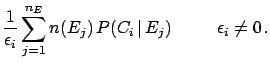
When inefficiency7.2
is also brought into the picture,
the best estimate of the true
number of events becomes
From these unfolded events we can estimate
the true total number of events,
the final probabilities of the causes and the overall efficiency:
If the initial distribution
 is not consistent with the
data, it will not agree with the final distribution
is not consistent with the
data, it will not agree with the final distribution
 .
The closer the initial distribution is to
the true distribution, the better
the agreement is.
For simulated data one can easily verify
that the distribution
lies between
and the true one. This suggests proceeding iteratively.
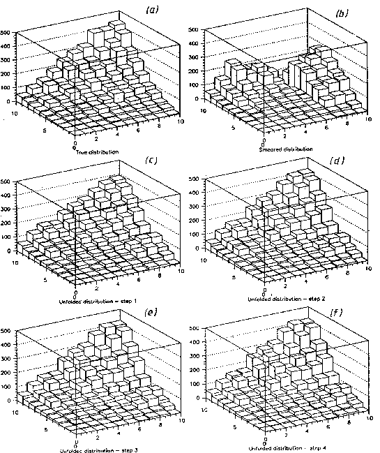
Fig. shows an example of a bidimensional distribution
unfolding.
.
The closer the initial distribution is to
the true distribution, the better
the agreement is.
For simulated data one can easily verify
that the distribution
lies between
and the true one. This suggests proceeding iteratively.
Fig. shows an example of a bidimensional distribution
unfolding.
More details about iteration strategy, evaluation of uncertainty,
etc. can be found in Ref. [56].
Figure:
Example of a two-dimensional unfolding: true distribution
(a), smeared distribution (b)
and results after the first four steps [(c) to (f)].
 |
I would just like to comment on an obvious criticism that may be made:
``the iterative procedure is against the Bayesian spirit, since
the same data are used many times
for the same inference''. In principle
the objection is valid, but in practice this
technique is a ``trick'' to give
to the experimental data a weight (an importance) larger than
that of the priors. A more rigorous procedure which took into
account uncertainties and correlations of the initial distribution
would have been much more complicated.
An attempt of this kind can be found in Ref. [57].
Examples of unfolding procedures performed with
non-Bayesian methods are described
in Refs. [54] and [55].
Note added: A recent book by Cowan[58] contains an interesting
chapter on unfolding.
Next: Other comments, examples and
Up: Bayesian unfolding
Previous: Bayes' theorem stated in
Contents
Giulio D'Agostini
2003-05-15