Next: Is there a signal?
Up: Poisson model: dependence on
Previous: Combination of results: general
Contents
Including systematic effects
A last interesting case is when there are systematic
errors of unknown size in the detector performance.
Independently of where
systematic errors may enter, the final result
will be an uncertainty on  . In the most general
case, the uncertainty can be described by a probability density function:
. In the most general
case, the uncertainty can be described by a probability density function:

best knowledge on experiment

For simplicity we analyse here only the case of a single experiment.
In the case of many experiments, we only need to iterate the Bayesian
inference, as has often been shown in these notes.
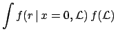
Following the general lines given in Section ![[*]](file:/usr/lib/latex2html/icons/crossref.png) ,
the problem can be solved by considering the conditional probability,
obtaining :
,
the problem can be solved by considering the conditional probability,
obtaining :
The case of absolutely precise knowledge of is recovered
when
 is a Dirac delta.
Let us treat in some more detail the case of null observation
(
 ). For each possible value of
one has an exponential of expected value
). For each possible value of
one has an exponential of expected value
 [see Eq. ()]. Each of the exponentials is weighted
with
. This means that, if
is rather symmetrical around its
barycentre (expected value), in a first approximation
the more and less steep exponentials will compensate, and the
result of integral () will be close to
[see Eq. ()]. Each of the exponentials is weighted
with
. This means that, if
is rather symmetrical around its
barycentre (expected value), in a first approximation
the more and less steep exponentials will compensate, and the
result of integral () will be close to  calculated in the barycentre of , i.e. in its
nominal value
calculated in the barycentre of , i.e. in its
nominal value
 :
:
 Data Data |
 |
 Data Data d d Data Data |
|
 Data Data |
 |
Data |
|
Figure:
Inference on the rate of a process, with and without
taking into account systematic effects:
upper plot: difference between
 and
and
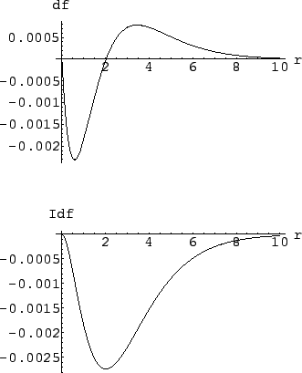 , using a normal
distribution of ; lower plot: integral of the
difference, to give a direct idea of the variation of the upper limit.
, using a normal
distribution of ; lower plot: integral of the
difference, to give a direct idea of the variation of the upper limit.
 |
To make a numerical example, let us consider
 (arbitrary units), with
following a
normal distribution.
The upper plot of
Fig. shows the difference between
(arbitrary units), with
following a
normal distribution.
The upper plot of
Fig. shows the difference between
 Data
Data calculated applying Eq.
() and the result obtained with the nominal
value
calculated applying Eq.
() and the result obtained with the nominal
value
 :
:
 is negative up to
 , indicating that systematic errors normally distributed
tend to
increase the upper limit.
But the size of the effect is
very tiny, and depends on the probability level
chosen for the upper limit.
This can be seen better in the lower plot of Fig.
,
which shows the integral of the difference of the two functions.
The maximum difference is for
.
As far as the upper limits are concerned, we obtain
(the large number of -- non-significatant--digits is only to observe
the behaviour in detail):
, indicating that systematic errors normally distributed
tend to
increase the upper limit.
But the size of the effect is
very tiny, and depends on the probability level
chosen for the upper limit.
This can be seen better in the lower plot of Fig.
,
which shows the integral of the difference of the two functions.
The maximum difference is for
.
As far as the upper limits are concerned, we obtain
(the large number of -- non-significatant--digits is only to observe
the behaviour in detail):
An uncertainty of 10% due to systematics produces only a
1% variation of the limits.
To simplify the calculation (and also to get a feeling of what
is going on) we can use some approximations.
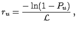
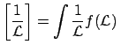
- Since the dependence of the upper limit of
 from
is given by
the upper limit averaged with the belief on is
given by
We need to solve an integral simpler than in the previous case.
For the above example of
we obtain
from
is given by
the upper limit averaged with the belief on is
given by
We need to solve an integral simpler than in the previous case.
For the above example of
we obtain
 at 90% and
 at 95%.
- Finally, as a real rough approximation, we can take into account
the small asymmetry of
 around the value obtained at the
nominal value of averaging the two values
of at
around the value obtained at the
nominal value of averaging the two values
of at
 from
:
from
:
We obtain numerically identical results to the previous approximation.
The main conclusion is that
the uncertainty due to systematics plays only a second-order role,
and it can be neglected for all practical purposes.
A second observation is that this uncertainty increases slightly
the limits if
is distributed normally, but
the effect could also be negative if the
is asymmetric
with positive skewness.
As a more general remark, one should not forget that
the upper limit has the meaning of an uncertainty and not of a
value of quantity.
Therefore, as nobody really cares about an uncertainty of 10 or 20%
on the uncertainty, the same is true for upper/lower limits.
At the per cent level it is mere numerology (I have calculated it at
the 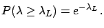 level just for mathematical curiosity).
Next: Is there a signal?
Up: Poisson model: dependence on
Previous: Combination of results: general
Contents
Giulio D'Agostini
2003-05-15
 E
E