Next: Including other experiments
Up: Constraining the mass of
Previous: Interpretation of the results
Contents
With the Bayesian method it is possible to trace the point in which
an unstated condition has been introduced, and how to remove it, or
how to take it into account.
With the form of the likelihood used in (![[*]](file:/usr/lib/latex2html/icons/crossref.png) ) it was
implicit that
) it was
implicit that  should not exceed
  . A more physically motivated
likelihood should be:
. A more physically motivated
likelihood should be:
![$\displaystyle f(x=0\,\vert\,m) = \left\{ \begin{array}{lcl} \exp{\left[-k\,\lef...
...ht]} & \mbox{if} & 0\le m\le E_b \\ 1 & \mbox{if} & m > E_b \end{array} \right.$](img1533.png) |
(9.24) |
Taking a uniform prior, we get the following posterior:
 |
(9.25) |
where
 comes from the integral
 .
So, we get our solution () for
.
So, we get our solution () for
 .
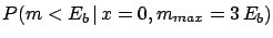
In general, the probability that
.
In general, the probability that  is smaller than 1
and decreases for increasing
is smaller than 1
and decreases for increasing  . For the parameters
of experiment
. For the parameters
of experiment  the integral in the denominator is equal
to 0.0058. Therefore, if, for example,
the integral in the denominator is equal
to 0.0058. Therefore, if, for example,
There is another reasoning which leads to the same conclusion.
At 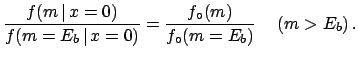 the detector has zero sensitivity.
For this reason, in case of null observation, this values gets the
maximum degree of belief. As far as larger values are concerned,
the odds ratios with respect to must be invariant,
since they are not influenced by the experimental observations, i.e.
the detector has zero sensitivity.
For this reason, in case of null observation, this values gets the
maximum degree of belief. As far as larger values are concerned,
the odds ratios with respect to must be invariant,
since they are not influenced by the experimental observations, i.e.
 |
(9.26) |
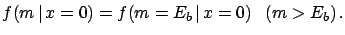
Since we are using, for the moment, a uniform distribution, the
condition gives:
 |
(9.27) |
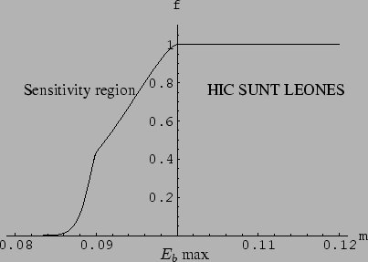
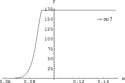
Figure:
Result of the inference from experiment ,
taking into account values of mass above the beam energy as well.
These all have the same degree of belief and the normalization constant
depends on the maximum value of considered. Therefore the distribution
is usually improper.
 |
We easily get the result shown in
Fig. by this piece of Mathematica code:
(********************************************************)
famax=fa/.m->eba
f2a=If[m<eba, fa, famax]

(* f2a(m) represents instead the (improper) distribution
   extended also for values larger that eba, in the light
   of a flat prior and of the Experiment A *)

Plot[f2a, {m,0.06,0.15}]
(********************************************************)
The curve is extended on the right side up to a limit
which cannot be determined by this experiment,
it could virtually go to infinity. For this reason the ratio
of probabilities
decreases
(i.e. we tend to believe more strongly large mass values)
but its exact value is not
well defined. For this reason we leave the function `open'
on the right side and unnormalized. The normalization will
be done when we can include other data which can provide
an upper limit.
Next: Including other experiments
Up: Constraining the mass of
Previous: Interpretation of the results
Contents
Giulio D'Agostini
2003-05-15