Including other experiments

Each of the other experiments are treated in exactly the same way. Comparing $B$ and $C$ it is interesting to see how the beam energy and the sensitivity factor contribute to constraining the mass. For reasons of space the plots are not shown. This is the rest of the Mathematica code to conclude the analysis:

(********************************************************)
(* Experiment B has been run at beam energy 0.09, with 
   sensitivity factor k=100,  threshold function beta^3, and 
   has observed 0 events.*)    

kb=100
ebb=0.09
v=Sqrt[1-(m/ebb)^2]
lambda= kb*v^3
lik=Exp[-lambda]
norm=NIntegrate[lik, {m, 0, ebb}]
fb=lik/norm
avb = NIntegrate[m*fb, {m, 0, ebb}]
Plot[fb, {m, 0.07, ebb}, PlotRange->{0, 600}, 
     AxesLabel -> {m, f}]

fbmax=fb/.m->ebb
f2b=If[m<ebb, fb, fbmax]
Plot[f2b, {m,0.07,0.15},  PlotRange->{0, 600},
     AxesLabel -> {m, f}]

(* The conclusions from A + B are, with and without the condition m<ebeam, 
   respectively (remember that the latter is improper): *)

fcom1ab=fa*fb/NIntegrate[fa*fb, {m, 0, eba}]
avab = NIntegrate[m*fcom1ab, {m, 0, eba}]               
Plot[fcom1ab, {m, 0.07, eba},  PlotRange->{0, 600},
     AxesLabel -> {m, f}]
fcom2ab=f2a*f2b

(* Experiment C has been run at beam energy 0.1, with sensitivity factor k=10, 
   threshold function beta^3 and, has observed 0 events. *)   

kc=10
ebc=0.1
v=Sqrt[1-(m/ebc)^2]
lambda= kc*v^3
lik=Exp[-lambda]
norm=NIntegrate[lik, {m, 0, ebc}]
fc=lik/norm
Plot[fc, {m, 0.07, ebc}, PlotRange->{0, 100},
     AxesLabel -> {m, f}]
avc = NIntegrate[m*fc, {m, 0, ebc}]
fcmax=fc/.m->(ebc-0.000001)
f2c=If[m<ebc, fc, fcmax]
Plot[f2c, {m,0.07,0.15},  PlotRange->{0, 100}, 
     AxesLabel -> {m, f}]
(********************************************************)

Figure: Final distribution (improper, see text) on $m$ from experiments $A$, $B$ and $C$. The curve has been arbitrarily rescaled to have the maximum of 1.

The combination of the result is done in the usual way, multiplying the likelihoods or the final p.d.f.'s, if these were obtained from a uniform distribution. We only see the combination of the three experiments, shown in Fig. . Finally, the indirect determinations are also included.

 
(********************************************************)
(* Conclusions from A + B + C , with and without the condition m<ebeam, 
   respectively (remember that the latter is improper): *)

fcom1abc=f2a*f2b*fc/NIntegrate[f2a*f2b*fc, {m, 0, ebc}]
avabc=NIntegrate[m*fcom1abc, {m, 0, ebc}]
Plot[fcom1abc, {m, 0.07, ebc},  PlotRange->{0, 150}, 
     AxesLabel -> {m, f}]
fcom2abc=f2a*f2b*f2c

(* Now we add independent determinations of m, 
   deriving from normal likelihoods, 
   and assuming uniform prior *)

g1=1/sigma1/(Sqrt[2*Pi])*Exp[-(m-mu1)^2/2/sigma1^2]
g2=1/sigma2/(Sqrt[2*Pi])*Exp[-(m-mu2)^2/2/sigma2^2]

mu1=0.09
sigma1=0.04
mu2=0.15
sigma2=0.04

(* The two overall (improper) priors may be a uniform, 
   or 1/m, i.e.  flat in ln(m), to express initial  
   uncertainty on the order of magnitude of m *)

p1=1
p2=1/m

final1=fcom2abc*g1*g2*p1/NIntegrate[fcom2abc*g1*g2*p1, {m, 0, 10}]
mean1=NIntegrate[m*final1, {m, 0, 10}] 
std1=Sqrt[NIntegrate[m^2*final1, {m, 0, 10}]-mean1^2]
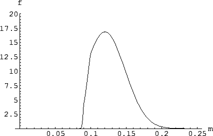
Plot[final1, {m, 0.0, 0.25},  PlotRange->{0, 20},
     AxesLabel -> {m, f}]

final2=fcom2abc*g1*g2*p2/NIntegrate[fcom2abc*g1*g2*p2, {m, 0, 10}]
mean2=NIntegrate[m*final2, {m, 0, 10}] 
std2=Sqrt[NIntegrate[m^2*final2, {m, 0, 10}]-mean2^2]
Plot[final2, {m, 0.0, 0.25},  PlotRange->{0, 20}, 
     AxesLabel -> {m, f}]
(********************************************************)

Finally, the two extra pieces of information enable us to constrain the mass also on the upper side and to arrive at a proper distribution (see Fig. ), under the condition that $H$ exists.

From the final distribution we can evaluate, as usual, all the quantities that we find interesting to summarize the result with a couple of numbers. For a more realistic analysis of this problem see Ref. [26].

Figure: Final mass distribution using all five pieces of experimental information, and assuming uniform priors. The curve obtained from the prior $1/m$ does not differ substantially from this.