From a sample of individual observations to a
couple of numbers: the role of
statistical sufficiency
Let us restart from the Eq. (5) of Ref. [2],
based on the graphical model in Fig. 5 of the same paper,
reproduced here for the reader's convenience
as Eq. (1) and Fig. 1.
Figure:
Graphical model behind the standard combination,
assuming independent measurements of the same quantity, each
characterized by a Gaussian error function with standard deviation

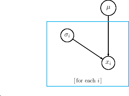 |
is the joint probability density function (pdf) of all the
quantities of interest,
with
 . The standard deviations
 are instead considered just conditions of the problem.
The pdf
are instead considered just conditions of the problem.
The pdf  models our prior beliefs about the `true' value
of the quantity of interest (see Ref. [2]
for details, in particular footnote 9). The pdf of
models our prior beliefs about the `true' value
of the quantity of interest (see Ref. [2]
for details, in particular footnote 9). The pdf of  , also
conditioned
on
, also
conditioned
on  , is then, in virtue of a well known theorem of
probability theory,
, is then, in virtue of a well known theorem of
probability theory,
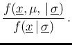
Noting that, given the model and the observed values
,
the denominator is just a number, although in general
not easy to calculate,
and making use of Eq. (1), we get
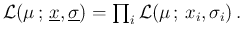
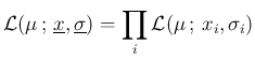
Speaking in terms of likelihood, and ignoring
multiplicative factors,5we can rewrite the previous equation as
that is, indeed, the particular case, valid for independent
observations  , of the more general form
since, under condition of independence,
- The inference depends on the product of likelihood and prior
(note `;' instead of `
 ' in the notation,
to remind that in `conventional statistics'
' in the notation,
to remind that in `conventional statistics'
 is simply a mathematical
function of , with parameters and
is simply a mathematical
function of , with parameters and
 );
);
- if the prior is `flat',6then the inference is determined by the likelihood,
In particular,
the most probable value7(`mode') of is the value which maximizes
the likelihood;8
- in the case of independent Gaussian error functions
the likelihood can be rewritten, besides multiplicative factors,
as
having recognized the sum in the exponent
as
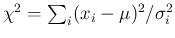 :
under the hypotheses and the approximations of this model the most probable
value of can then also be obtained by
minimizing
:
under the hypotheses and the approximations of this model the most probable
value of can then also be obtained by
minimizing  ; 9
; 9
- going through the steps from Eqs. (7)-(12) of
Ref. [2] and, under
the assumptions stated in the previous items,
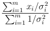
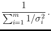
we can further rewrite the Eq. (3) as
where
in which we recognize Gauss' Eqs. (G1) and (G2).
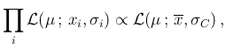
In terms of likelihoods,
Equation (7) is an important result, related
to the concept of
statistical sufficiency: the inference is exactly the same
if, instead of using the detailed information provided by
and
 , we just
use the weighted mean
, we just
use the weighted mean  and its
standard deviation
and its
standard deviation  , as if
  were
a single equivalent observation of with a Gaussian error function
with “degree of accuracy” [1]
were
a single equivalent observation of with a Gaussian error function
with “degree of accuracy” [1]  -
this is exactly the result Gauss was aiming in Book 2, Section 3 of
Ref. [1], reminded in the opening quote
and in the introduction
of Ref. [2].
-
this is exactly the result Gauss was aiming in Book 2, Section 3 of
Ref. [1], reminded in the opening quote
and in the introduction
of Ref. [2].
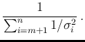
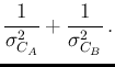
Moreover we can split the sum of Eq.(3)
in two contributions,
from  to
to  (arbitrary) and from
  to
to  , thus having
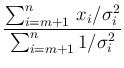
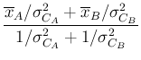
Going again through the steps from Eq.(7) to Eq.(12) of
Ref. [2] we get
where
It follows, writing the right hand side as product of exponentials
and complementing each of them [2],
that is, in terms of likelihoods,
The result can be extended to averages of averages, that is
where
The property can be extended further to many partial averages,
showing that the inference
does not depend on whether we use the individual
observations, their weighted average or even the grouped weighted
averages, or the weighted average of the grouped averages.
This is one of the `amazing' properties
of the Gaussian distribution, which simplifies our work
when it is possible to use it.
But there no
guarantee that it works in general, and it should be
then proved case by case.
![\begin{eqnarray*}
f(\mu\,\vert\,\underline{x},\underline{\sigma}) &\propto&
\left[ \prod_i f(x_i\,\vert\,\mu,\sigma_i)\right]\cdot f_0(\mu) %
\end{eqnarray*}](img32.png)
![\begin{eqnarray*}
f(\mu\,\vert\,\underline{x},\underline{\sigma}) &\propto&
\l...
... \prod_i {\cal L}(\mu\,;\,x_i,\sigma_i) \right]\cdot f_0(\mu)\,,
\end{eqnarray*}](img33.png)
![$\displaystyle \exp\left[-\sum_i\,\frac{(x_i-\mu)^2}{2\,\sigma_i^2}\right]$](img44.png)
![$\displaystyle \exp\left[- \frac { (\mu-\overline{x})^2}{2\,\sigma_C^2}\right] \,,$](img47.png)
![$\displaystyle \exp\left[-\sum_{i=1}^{m}\,\frac{(x_i-\mu)^2}{2\,\sigma_i^2}
-\sum_{i=m+1}^{n}\,\frac{(x_i-\mu)^2}{2\,\sigma_i^2} \right]\,.$](img63.png)
![$\displaystyle \exp\left[- \frac{ - 2\,\overline{x}_A\,\mu
+ \mu^2}{2\,\sigma_{C_A}^2} -
\frac{ - 2\,\overline{x}_B\,\mu
+ \mu^2}{2\,\sigma_{C_B}^2}
\right]$](img64.png)
![$\displaystyle \exp\left[- \frac { (\overline{x}-\mu)^2}
{2\,\sigma_C^2} \right]$](img73.png)
![$\displaystyle \exp\left[- \frac { (\overline{x}_{A}-\mu)^2}
{2\,\sigma_{C_A}^2}...
...\cdot
\exp\left[- \frac { (\overline{x}_{B}-\mu)^2}
{2\,\sigma_{C_B}^2} \right]$](img74.png)
![$\displaystyle \exp\left[- \frac { (\overline{x}_{A}-\mu)^2}
{2\,\sigma_{C_A}^2} - \frac { (\overline{x}_{B}-\mu)^2}
{2\,\sigma_{C_B}^2} \right]\,,$](img75.png)
![$\displaystyle \left[ \prod_i f(x_i\,\vert\,\mu,\sigma_i)\right]\cdot f_0(\mu)\,$](img24.png)
![$\displaystyle \prod_i \exp\left[-\frac{(x_i-\mu)^2}{2\,\sigma_i^2}\right]$](img43.png)