Possibly discrepant results

Well known features of the combination of measurements by the weighted average, reminded in the last section, are that i) the combined result has a “degree of precision” [1] higher than each of the individual contributions or, in terms of standard deviations, $\sigma_C < \sigma_i$ ; ii) the resulting standard deviation does not depend on the spread of the individual results around the mean value; iii) the error model of the `equivalent observation' remains Gaussian. However, it is a matter of fact that, although from the probabilistic point of view there is no contradiction with the basic assumptions, since patterns of individual results `oddly' scattered around their average have some chance to occur, we sometimes suspect that there it might be something `odd' going on. That is, we tend to doubt on the validity of the simple model of Gaussian errors with the declared “degrees of precision”. (But someone might start to worry too early,¹⁰ sometimes even driven by wishful thinking, that is she hopes, rather than believes, that the reason of disagreement might be caused by new phenomenology or violation of fundamental laws of physics [8,9].)

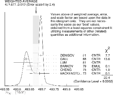
**Figure:** Charged kaon mass from several experiments as summarized by the PDG [7]. Note that besides the `error' of 0.013 MeV, obtained by a $\times 2.4$ scaling, also an `error' of 0.016 MeV is provided, obtained by a $\times 2.8$ scaling. The two results are called `OUR AVERAGE' and 'OUR FIT', respectively [7].
$\begin{figure}\centering\epsfig{file=PDG_summary.eps,clip=,width=0.7\linewidth}\end{figure}$

In the case we have serious suspicions about the presence of other effects, then we should change our model, make a new analysis and accept its outcome in the light of clearly stated hypotheses and conditions [2,3,4]. As a result, not only the overall `error'¹¹ should change, but also the shape of the final distribution should, since there is no strong reason to remain Gaussian. For example, the final distribution might be skewed or even multimodal [2], as it should be desirable if the pattern of individual measurements suggest so. In particular, the most probable value (mode) will differ from the average of the distribution and from the median. Instead, traditionally, only the `error' is enlarged by an arbitrary factor depending on the frequentistic `test variable' $\chi ^2$ , namely $\sqrt {\chi ^2/\nu }$ , where $\nu$ stands for the number of degrees of freedom. But the central value is kept unchanged and the interpretation of the result, explicitly stated or implicitly assumed so in subsequent analyses by other scientists, remains Gaussian.¹²

Table: Experimental values of the charged kaon mass used in the numerical example, limited to those taken into account by the 2019 issue of PDG [7]. (*) `error' already scaled by a factor $\times 1.52$ due to the $\sqrt {\chi ^2/\nu }$ prescription (see text). (**) Value accepted by the PDG.

Authors	pub. year	central value	uncertainty
		(MeV)	(MeV)
G. Backenstoss et al. [14]	1973	493.691	0.040
S.C. Cheng et al. [15]	1975	493.657	0.020
L.M. Barkov et al.[16]	1979	493.670	0.029
G.K. Lum et al. [17]	1981	493.640	0.054
K.P. Gall et al. [18]	1988	493.636	0.011 (*)
A.S. Denisov et al. [19]	1991	493.696	0.0059
& Yu.M. Ivanov [20]	1992	same	0.007 (**)

As a practical example, let us take the results concerning the charged kaon mass of Fig. 2 and Tab. 1, as selected by the PDG [7].

**Figure:** Graphical representation of the results on the charged kaon mass of Tab. 1 (solid blue Gaussians). The dashed red Gaussian shows the result of the standard combination obtained by the weighted average. The solid gray Gaussian, centered with the dashed red one, shows the broadening due to the $\sqrt {\chi ^2/\nu }$ prescription (see text).
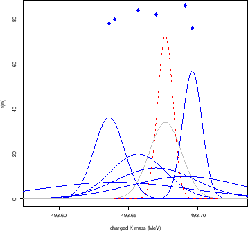$\begin{figure}\centering\epsfig{file=naive_combination_curious.eps,clip=,width=0.65\linewidth}\end{figure}$

From the weighted average and its standard deviation we get $493.6766 \pm 0.0055\,$ MeV, shown in Fig. 3 by the dashed red Gaussian (the solid blue Gaussians depict the results of the six results of Tab. 1. Comparing the individual results with the weighted average we calculate a $\chi ^2$ of 22.9, and hence a scaling factors of 2.14, getting then $493.677 \pm 0.012\,$ MeV, reported on the same figure by the solid gray Gaussian below the dashed one.¹³The two results are reported also in the entry A of the summary table 3.