Reasons of dissatisfaction with the $\chi ^2$-motivated scaling prescription

As we see in Fig. 3, the Gaussian widened by the $\sqrt {\chi ^2/\nu }$ prescription does not capture the picture offered by the ensemble of the individual results. In fact, the mass values preferred by the combined result are still distributed symmetrically around the weighted average.¹⁴

More in general, the scaling factor is at least suspect. This is because it is well known that the $\chi ^2$ distribution does not scale with $\nu$ and therefore, while a $\chi/\nu = 2$, for example, is quite in the norm for $\nu$ equal to 2, 3 or 4 (even a strict frequentist would admit that the resulting p-values of 0.14, 0.11 and 0.09, respectively, are nothing to worry), things get different for $\nu$ equal to 10, 20 or 30 (p-values of 0.029, 0.005 and 0.0009, respectively). Moreover, I am not aware of cases in which the standard deviation of the weighted average was scaled down, in the case that $\sqrt {\chi ^2/\nu }$ was smaller than one.¹⁵

But there is another subtle issue with the method, which I have realized only very recently, going through the details of the charged kaon mass measurements: if the prescription is applied to a sub-sample of results and then to all them (taking for the sub-sample weighted average and scaled standard deviation), then a bias is introduced in the final result with respect to when all results were taken individually. This is because the summary provided by such a prescription is not a sufficient statistics.

The lowest, high precision mass value of $493.636 \pm 0.011$ (see Tab. 1 and Fig. 3) come in fact from the combination, done directly by the experimental team [18] applying the $\sqrt {\chi ^2/\nu }$ prescription. Without this scaling, the four individual results, reported in Tab. 2,

Table: Individual results reported by [18], together with their combination.

	Authors	pub. year	$[d_i]$	$[s_i]$
$i$			(MeV)	(MeV)
$5_a$	K.P. Gall et al. [18]	1988	493.675	0.026
$5_b$			493.631	0.007
$5_c$			493.806	0.095
$5_d$			493.709	0.073
$5$	K.P. Gall et al. [18]	1988	493.636	0.011

Table: Combinations of the individual results of Tabs. 1 and 2. The subscript $S$ means that the $\sqrt {\chi ^2/\nu }$ scaling prescription has been applied to standard deviation of the weighted average. In particular, note that $\{1,2,3,4,5,6\}_S$ is the same as $\{1,2,3,4,\{5_a,5_b,5_c,5_d\}_S,6\}_S$.

	data set	$m_{K^\pm}$/MeV
<#2410#>	$\{1,2,3,4,5,6\}$	$493.6766\pm0.0055$
		$\{1,2,3,4,5,6\}_S$
<#2415#>	$\{5_a, 5_b, 5_c, 5_d\}$	$493.6355\pm 0.0067$
		$\{5_a, 5_b, 5_c, 5_d\}_S$
<#2420#>	$\{1,2,3,4,5_a,5_b,5_c,5_d,6\}$	$493.6644\pm 0.0046$
		$\{1,2,3,4,5_a,5_b,5_c,5_d,6\}_S$
<#2425#>	$\{1,2,3,4,5_a,5_b,5_c,5_d\}$	$493.6404\pm 0.0061$
		$\{1,2,3,4,5_a,5_b,5_c,5_d\}_S$
<#2430#>	$\{\{1,2,3,4,5_a,5_b,5_c,5_d\}_S,6\}$	$493.6705\pm 0.0051$
		$\{\{1,2,3,4,5_a,5_b,5_c,5_d\}_S,6\}_S$

had given a weighted average of $493.6355 \pm 0.0067\,$MeV, with a $\chi ^2$ of 7.0. Now it is true that $\chi^2/\nu$ is equal to 2.32, but this is not a reason to worry, being $\nu=3$. In fact the p-value, calculated as $P(\chi^2\,\vert\,\nu=3) > 7.0$, is 0.073, that is even above the (in-)famous 0.05 threshold [9].

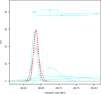
Nevertheless, if we apply to the standard deviation a scaling factor of $\sqrt{2.32} = 1.52$, then we get $493.636 \pm 0.010\,$MeV (the difference between this value of 0.010 MeV and 0.011 MeV of Tabs. 1 and 2 could be just due to rounding of the individual values). The result is shown in Fig. 4, together with the individual results that enter the analysis (see also entry B of the summary table 3).

Figure: Individual results of Ref. [18] (cyan solid lines), with the weighted average with and without $\sqrt {\chi ^2/\nu }$ scaling factor (same graphic notation of Fig. 3).

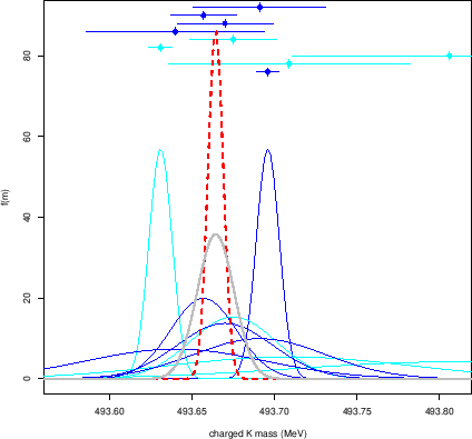
It is interesting to see what we get if we use the nine individual points, i.e. 1, 2, 3, 4 and 6 of Tab. 1, together with $5_a$, $5_b$, $5_c$ and $5_d$ of Tab. 2.

Figure: Combination of the individual results of Ref. [18], together with the other results (i.e. excluding nr. $5$) of Tab. 1. For details of the graphic notation see the previous figures.

The combined weighted average, shown in Fig. 5, comes out right in the middle of the two most precise results, with little overlap with them. The average is $493.6644\,$MeV, with standard deviation $0.0046\,$MeV, which becomes $0.011\,$MeV after the $\chi ^2$ motivated scaling¹⁶ of $\times 2.42$. As we can see, the central value differs by $-12\,$keV with respect from the one obtained above $[$ see also section. 3 and entry C of the summary table 3 $]$: the use of the pre-combined result of Ref. [18] produces a bias of $+12\,$keV in the final result, that is comparable with the quoted `error'. The reason is due to the fact that the $\sqrt {\chi ^2/\nu }$ prescription used to enlarge the standard deviation does not hold sufficiency. As a consequence, the relevance of the ensemble of results of Ref. [18] gets reduced.

As a further example to show this effect on the same data, let us make the academic exercise of grouping the data in a different way. For example we first combine all results published before year 1990 (1-4,$5_a$-$5_d$, with references to Tabs.  1 and 2, and include the most recent one (6 of Tab. 1) in a second step. The outcome of the exercise is reported in Fig. 6 and in the entries D and E of the summary table 3.

Figure: Example of arbitrary grouping of the results in before and after year 1990 (see text).

The weighted average of the eight results before year 1990 (upper plot of Fig. 6 and entry D in Tab. 3) gives $m_{K^\pm} = 493.6404\pm0.0061\,$MeV (dashed red line). The $\chi ^2$ is equal to 10.8, producing a scaling factor of 1.24 and thus a modified result of $m_{K^\pm} = 493.6404\pm0.0076\,$MeV (solid brown line of Fig. 6 and entry D in Tab. 3).

Combining this outcome with the 1991 result [19,20] we get (lower plot of Fig. 6 and entry E in Tab. 3) a weighted average of $m_{K^\pm} = 493.6705\pm 0.0051\,$MeV, but with the very large $\chi ^2$ of 29 (p-value $0.74\times 10^{-7}$), thus yielding a $\times 5.4$ scaling factor and then a widened standard deviation of $28\,$keV. At least, contrary to the previous cases, this time the scaled standard deviation is able to cover both individual results, although an experienced physicist would suspect that most likely only one of the two is correct. (In situations of this kind a `sceptical analysis' would result in a bimodal distribution, as shown in Fig. 4 of Ref. [3].)