The binomial distribution and its inverse problem

An important class of counting experiments can be modeled as independent Bernoulli trials. In each trial we believe that a success will occur with probability $p$, and a failure with probability $q=1-p$. If we consider $n$ independent trials, all with the same probability $p$, we might be interested in the total number of successes, independently of their order. The total number of successes $X$ can range between $0$ and $n$, and our belief on the outcome $X=x$ can be evaluated from the probability of each success and some combinatorics. The result is the well known binomial distribution, hereafter indicated with ${\cal B}_{n,p}$:

$$f(x\,\vert\,{\cal B}_{n,p}) = \frac{n!}{(n-x)!\,x!}\, p^x\, ... ... 0 \le p \le 1 \\ x = 0, 1, \ldots, n \end{array}\right.\,,$$ (1)

having expected value and standard deviation

$$\mbox{E}(X) = n\,p$$ (2)

$$\sigma(x) = \sqrt{n\,p\, (1-p)}\,.$$ (3)

We associate the formal quantities expected value and standard deviation to the concepts of (probabilistic) prevision and standard uncertainty.

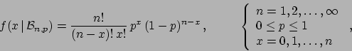
The binomial distribution describes what is sometimes called a direct probability problem, i.e. calculate the probability of the experimental outcome $x$ (the effect) given $n$ and an assumed value of $p$. The inverse problem is what concerns mostly scientists: infer $p$ given $n$ and $x$. In probabilistic terms, we are interested in $f(p\,\vert\,n,x)$. Probability inversions are performed, within probability theory, using Bayes theorem, that in this case reads

$$f(p\,\vert\,x,n,{\cal B}) \propto f(x\,\vert\,{\cal B}_{n,p}) \cdot f_\circ(p)\,$$ (4)

where $f_\circ(p)$ is the prior, $f(p\,\vert\,x,n,{\cal B})$ the posterior (or final) and $f(x\,\vert\,{\cal B}_{n,p})$ the likelihood. The proportionality factor is calculated from normalization. [Note the use of $f(\cdot)$ for the several probability functions as well as probability density functions (pdf), also within the same formula.] The solution of Eq. (4), related to the names of Bayes and Laplace, is presently a kind of first text book exercise in the so called Bayesian inference (see e.g. Ref. [2,3]). The issue of priors in this kind of problems will be discussed in detail in Sec. 3.1, especially for the critical cases of $x=0$ and $x=n$.

The problem can be complicated by the presence of background. This is the main subject of this paper, and we shall focus on two kinds of background.

a)

Background can only affect ${\mathbf x}$. Think, for example, of a person shooting $n$ times on a target, and counting, at the end, the numbers of scores $x$ in order to evaluate his efficiency. If somebody else fires by mistake at random on his target, the number $x$ will be affected by background. The same situation can happen in measuring efficiencies in those situations (for example due to high rate or loose timing) in which the time correlation between the equivalents of `shooting' and `scoring' cannot be done on a event by event basis (think, for example, to neutron or photon detectors).

The problem will be solved assuming that the background is described by a Poisson process of well known intensity $r_b$, that corresponds to a well known expected value $\lambda_b$ of the resulting Poisson distribution (in the time domain $\lambda_b=r_b\cdot T$, where $T$ is measuring time). In other words, the observed $x$ is the sum of two contributions: $x_s$ due to the signal, binomially distributed with ${\cal B}_{n,p}$, plus $x_b$ due to background, Poisson distributed with parameter $\lambda_b$, indicated by ${\cal P}_{\lambda_b}$.

For large numbers (and still relatively low background) the problem is easy to solve: we subtract the expected number of background and calculate the proportion $\hat p = (x-\lambda_b)/n$. For small numbers, the `estimator' $\hat p$ can become smaller than 0 or larger then 1. And, even if $\hat p$ comes out in the correct range, it is still affected by large uncertainty. Therefore we have to go through a rigorous probability inversion, that in this case is given by

$$f(p\,\vert\,n,x,\lambda_b) \propto f(x=x_s+x_b\,\vert\,n,p,\lambda_b) \cdot f_\circ(p) \,,$$ (5)

where we have written explicitly in the likelihood that $x$ is due to the sum of two (individually unobservable!) contributions $x_s$ and $x_b$ (hereafter the subscripts $s$ and $b$ stand for signal and background.)

b)

The background can show up, at random, as independent `fake' trials, all with the same ${\mathbf p_b}$ of producing successes. An example, that has indeed prompted this paper, is that of the measuring the proportion of blue galaxies in a small region of sky where there are galaxies belonging to a cluster, as well as background galaxies, the average proportion of blue galaxies of which is well known. In this case both $n$ and $x$ have two contributions:

$$n = n_s+n_b$$ (6)

$$x = x_s+x_b$$ (7)

with

$$n_b \sim {\cal P}_{\lambda_b}$$ (8)

$$x_b \sim {\cal B}n_b,p_b$$ (9)

$$x_s \sim {\cal B}n_s,p_s\,,$$ (10)

where `$\sim$' stands for `follows a given distribution'.

Again, the trivial large number (and not too large background) solution is the proportion of background subtracted numbers, $\hat p = (x-p_b\,\lambda_b)/(n-\lambda_b)$. But in the most general case we need to infer $p$ from

$$f(p_s\,\vert\,n,x,\lambda_b,p_b) \propto f(x=x_s+x_b\,\vert\,n=n_s+n_b,p_b,\lambda_b) \cdot f_\circ(p) \,.$$ (11)

We might be also interested also to other questions, like e.g. how many of the $n$ object are due to the signal, i.e.

$$f(n_s\,\vert\,n,x,\lambda_b,p_b)\,.$$

Indeed, the general problem lies in the joint inference

$$f(n_s,p_s\,\vert\,n,x,\lambda_b,p_b),$$

from which we can get other information, like the conditional distribution of $p_s$ for any given number of events attributed to signal:

$$f(p_s\,\vert\,n,n_s,x,\lambda_b,p_b)\,.$$

Finally, we may also be interested in the rate $r_s$ of the signal objects, responsible of the $n_s$ signal objects in the sample (or, equivalently, to the Poisson distribution parameter $\lambda _s$):

$$f(\lambda_s\,\vert\,n,x,\lambda_b,p_b)\,.$$