Next: Inferring
Up: Inferring the success parameter
Previous: Uncertainty on the expected
Poisson background on the observed number of `trials'
and of `successes'
Let us know move to problem b) of the introduction.
Again, we consider only the background parameters are well
known, and refer to the previous subsection for treating
their uncertainty.
To summarize, that is what we assume to know with certainty:

- : the total observed numbers of `objects',
 of which
are due to signal and
of which
are due to signal and  to background; but these
two numbers are not directly observable and can only be inferred;
to background; but these
two numbers are not directly observable and can only be inferred;

- : the total observed numbers of the `objects' of the
subclass of interest, sum of the unobservable
 and
and  ;
;

- : the expected number of background objects;

- : the expected proportion of successes
due to the background events.
As we discussed in the introduction, we are interested in inferring
the number of signal objects , as well as
the parameter  of the `signal'.
We need then to build a likelihood that connects the observed
numbers to all
quantities we want to infer. Therefore we need to calculate the
probability function
of the `signal'.
We need then to build a likelihood that connects the observed
numbers to all
quantities we want to infer. Therefore we need to calculate the
probability function
 .
.
Let us first calculate the probability function
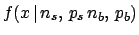 that depends on the unobservable and .
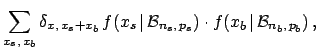
This is the probability function
of the sum of two binomial variables:
that depends on the unobservable and .
This is the probability function
of the sum of two binomial variables:
where ranges between  and ,
and ranges between and .
can vary between 0 and
and ,
and ranges between and .
can vary between 0 and  , has expected value
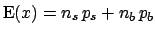 and variance
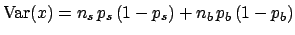 .
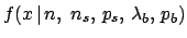
As for Eq. (32),
we need to evaluate
Eq. (35) only for the observed number of successes.
Contrary to the implicit convention within this paper
to use the same symbol
.
As for Eq. (32),
we need to evaluate
Eq. (35) only for the observed number of successes.
Contrary to the implicit convention within this paper
to use the same symbol  meaning different
probability functions and pdf's, we name Eq. (35)
meaning different
probability functions and pdf's, we name Eq. (35)
 for later convenience.
In order to obtain the general likelihood we need, two observations
are in order:
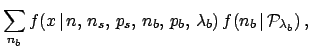
It follows that
At this point we get rid of in the conditions, taking
account its possible values and their probabilities, given :
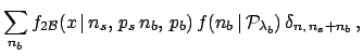
i.e.
where ranges between 0 and , due to the
 condition.
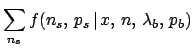
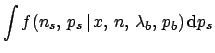
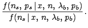
Finally, we can use Eq. (39) in Bayes theorem
to infer and :
condition.
Finally, we can use Eq. (39) in Bayes theorem
to infer and :
We give now some numerical examples. For simplicity (and because
we are not thinking to a specific physical case) we take
uniform priors, i.e.
 .
We refer to section 3.1 for an extensive discussion
on prior and on critical `frontier' cases.
.
We refer to section 3.1 for an extensive discussion
on prior and on critical `frontier' cases.
Subsections
Next: Inferring
Up: Inferring the success parameter
Previous: Uncertainty on the expected
Giulio D'Agostini
2004-12-13