Approximate methods and standard propagation applied to systematic errors

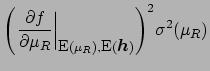
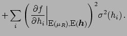
When we have many uncertain influence factors and/or the model of uncertainty is non-Gaussian, the analytic solution of Eq. (73), or Eqs. (77)-(79) can be complicated, or not existing at all. Then numeric or approximate methods are needed. The most powerful numerical methods are based on Monte Carlo (MC) techniques (see Sect. 9 for a short account). This issue goes beyond the aim of this report. In a recent comprehensive particle-physics paper by Ciuchini et al (2001), these ideas have been used to infer the fundamental parameters of the Standard Model of particle physics, using all available experimental information.

For routine use, a practical approximate method can be developed by thinking of the value inferred for the expected value of ${\mbox{\boldmath$h$}}$ as a raw value, indicated with $\mu_R$, that is, $\mu_R = \mu\left\vert _{ {\mbox{\boldmath$\scriptstyle h$}} \, = \, \mbox{\footnotesize E}({\mbox{\boldmath$\scriptstyle h$}})}\right.$ (`raw' in the sense that it needs later to be `corrected' for all possible value of ${\mbox{\boldmath$\theta$}}$, as it will be clear in a while). The value of $\mu$, which depends on the possible values of ${\mbox{\boldmath$h$}}$, can be seen as a function of $\mu_R$ and ${\mbox{\boldmath$h$}}$:

$$\mu = f(\mu_R, {\mbox{\boldmath$h$}})\,.$$ (85)

We have thus turned our inferential problem into a standard problem of evaluation of the pdf of a function of variables, of which are particularly known the formulae to obtain approximate values for expectations and standard deviations in the case of independent input quantities (following the nomenclature of ISO 1993):

$$\mbox{E}(\mu) \approx f(\mbox{E}(\mu_R), \mbox{E}({\mbox{\boldmath$h$}}))$$ (86)

$$\sigma^2(\mu) \approx \left(\left.\frac{\partial f}{\partial \mu_R}\right\vert _{\mbox{... ...l E}(\mu_R), \mbox{\small E}({\mbox{\boldmath$h$}})} \right)^2\!\sigma^2(\mu_R)$$

$$+ \sum_i \left(\left.\frac{\partial f} {\partial h_i}\right\vert ... ...(\mu_R), \mbox{\small E}({\mbox{\boldmath$h$}})} \right)^2\! \sigma^2(h_i) \, .$$ (87)

Extension to multi-dimensional problems and treatment of correlations is straightforward (the well-known covariance matrix propagation) and we refer to (D'Agostini and Raso 1999) for details. In particular, this reference contains approximate formulae valid up to second order, which allow to take into account relatively easily non linearities.