Probabilistic model

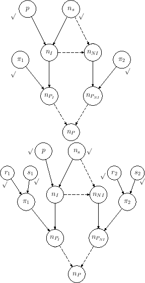
The graphical model describing the quantities of interest is shown in the left hand network of Fig. , based on that of Fig. , to which we have added parents to the nodes $n_I$ and $n_{NI}$, the number of Infected and Not Infected in the sample, respectively. More precisely, the number of infectees $n_I$ in the sample is described by a hypergeometric distribution, that is

$$n_I \sim (N_I,N_{NI},n_s)\,,$$

with $N_I$ and $N_{NI}$ the numbers of infected and not infected individuals in the population. Then, the number $n_{NI}$ of not infected people in the sample is deterministically related to $n_{I}$, being $n_{NI} = n_s - n_I$.

However, since in this paper we are interested in sample sizes much smaller than those of the populations, we can remodel the problem according to the right hand network of Fig. , in which $n_I$ is described by a binomial distribution, that is

$$n_I \sim (n_s, p)\,,$$

with $p=N_I/(N_I+N_{NI})$. This simplified model has been re-drawn in the network shown in the left hand side of Fig. ,

Figure: Simplified graphical model of Fig.  rewritten in order to make explicit `known'/`assumed' quantities, tagged by the symbol '$\surd\,$', and the uncertain ones. In particular, in the left hand diagram precise values of $\pi_1$ and $\pi_2$ are assumed, while in the the right hand one the uncertainty on their values is modeled with Beta pdf's with parameters $(r_1,s_1)$ and $(r_2,s_2)$.

indicating by the symbol `$\surd\,$' the certain variables in the game (indeed those which are for some reason assumed), in contrast to the others, which are uncertain and whose values will be ranked in degree of belief following the rules of probability theory. Note that in this diagram $\pi_1$ and $\pi_2$ are assumed to be exactly known. Instead, as we have already seen in Sec. , their values are uncertain and their probability distribution can be conveniently modeled by Beta probability functions characterized by parameters $r$'s and $s$'s. The graphical model which takes into account also the uncertainty about $\pi_1$ and $\pi_2$ is drawn in the same Fig.  (right side).

We have already discussed extensively, in Sec. , how the expectation of $n_P$, and therefore of the fraction on positives in the sample, $f_P$, depends on the model parameters. Now we go a bit deeper into the question of the dependence of $f_P$ on the fraction of infectees in the population and, more precisely, which are the `closest' (to be defined somehow) two values of $p$, such that the resulting $f_P$'s are `reasonably separated' (again to be defined somehow) from each other. Moreover, instead of simply relying on the approximated formulae developed in Sec. , we are going to use Monte Carlo methods in different ways: initially just based on R random number generators; then using (well below its potentials!) the program JAGS, which will then be used in Sec.  for inferences. However we shall keep using the approximated formulae for cross check and to derive some useful, although approximated, results in closed form.