Expected numbers of vaccinated individuals that shall become infected

Once we have got the efficacy of a vaccine, or, even better, the full information about $\epsilon$ inferred by the data, we can tackle another interesting problem: if we vaccinate

individuals in (possibly) another population, how many of them will become infected? Obviously, this depends not only on $f(\epsilon)$ but also on many other parameters that we can model with the assault probability

in the new population, and, obviously, on the fact that

must be only a small part of the entire population, so that we do not have to consider issues related to herd immunity. In order to do this exercise we need to enlarge our causal model, thus getting that shown in Fig.

**Figure:** *Variation of the model of Fig. , in this figure inside a box, in order to consider the effect of the vaccine on individuals of a different population (see text).*
$\begin{figure}\begin{center} \epsfig{file=vaccine_eff_pred.eps,clip=,width=0.8\linewidth} \\ \end{center} \end{figure}$

But in reality there is no need to set up a new JAGS model and rerun the MCMC. We can just use the chain of $\epsilon$ obtained processing through the MCMC the original model of Fig.

, and do the remaining work with `direct' Monte Carlo. However, having observed that the resulting pdf of $\epsilon$ is approximated a Beta, we can do it starting from the mean and standard deviation obtained from the MCMC. Here is e.g. how the evaluation of $n'_{V_I}$ can be performed by sampling (in the R code we have indicated

as nV, and so on):

mu <- 0.944; sigma <- 0.019; e.rep <- 0.950    # Pfizer
# mu <- 0.941; sigma <- 0.019; e.rep <- 0.941    # Moderna
# mu <- 0.861; sigma <- 0.075; e.rep <- 0.900    # AZ LDSD
# mu <- 0.599; sigma <- 0.090; e.rep <- 0.621    # AZ SDSD

# uncomment the following line to simulate a negligible uncertainty 
# sigma <- 0.0001   

r = (1-mu)*mu^2/sigma^2 - mu
s  = r*(1-mu)/mu
cat(sprintf("r = %.2f, s =  %.2f\n", r, s))

ns <- 1000000
nV <- 100000  
pA <- 0.01

nA <- rbinom(ns, nV, pA)
cat(sprintf("nA: mean+-sigma:  %.1f +- %.1f\n", mean(nA), sd(nA)))

eps <- rbeta(ns,r,s)
nvI <- rbinom(ns, nA, 1-eps)
hist(nvI, nc=100, col='cyan', freq=FALSE, main=”)
cat(sprintf("nvI: mean+-sigma:  %.1f +- %.1f\n", mean(nvI), sd(nvI)))
lines(rep(pA*nV*(1-mu), 2), c(0,1), col='red', lty=1, lwd=2)
lines(rep(pA*nV*(1-e.rep), 2), c(0,1), col='red', lty=2, lwd=2)

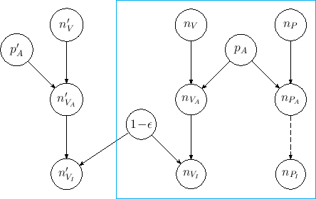
A number of hundred thousand vaccinated individuals has been used, with an absolutely hypothetical value of assault probability of 1 %. The script can also be used to simulate the effect of a precise value of 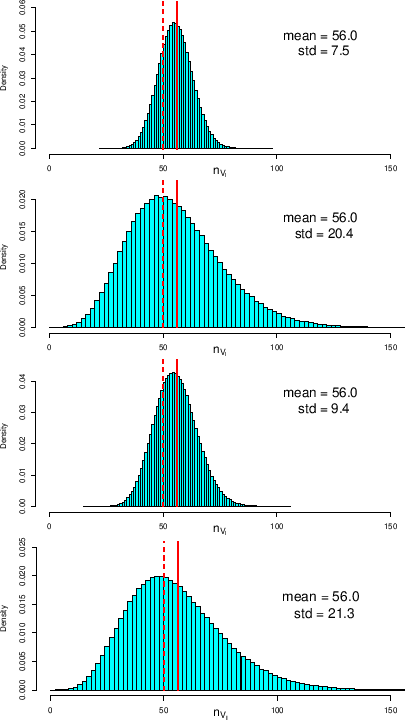$\epsilon$ , thus exactly corresponding to the efficacy, just setting its standard deviation to a very small value.

**Figure:** Distribution of the predicted number of vaccinated infectees, subject to (top-down): exact values of $\epsilon$ and ; uncertain $\epsilon$ ; uncertain ; uncertain $\epsilon$ and (see text for details).
$\begin{figure}\begin{center} \epsfig{file=predicted_VI_Pfizer_no_unc.eps,clip=,... ...73\linewidth} \\ \mbox{} \vspace{-1.3cm} \mbox{} \end{center} \end{figure}$

The result of this idealized situation, using e.g. $\epsilon = 0.944$ , i.e. the mean resulting from the MCMC analysis of Pfizer data,¹⁵is shown in the top histogram of Fig.

. In this idealized case the distribution of $n_{V_I}'$ is simply a binomial, i.e.

$\displaystyle n_{V_I}'$

$\displaystyle \sim$

Binom $\displaystyle (n_{V}',\, p_{ov})\,,$

with the overall probability $p_{ov}$ being equal to $p_A'\cdot(1\!-\!\epsilon)$ , that is $p_{ov} = 0.00056$ for the numbers reported in the script. Expected value and standard deviation are then 56.0 and 7.5, in perfect agreement with the Monte Carlo result shown in the upper panel of Fig.

The effect of the uncertainty about $\epsilon$ is shown in the second (top-down) histogram of the same figure. As we can see, the distribution becomes remarkably wider and more asymmetric, with a right-hand skewness, effect of the left-hand skewness of $f(\epsilon)$ . We see then, in the third histogram, the effect of a hypothetical uncertainty about , modeled here with a standard deviation of $\sigma(p'_A)=0.1\times p'_A$ (but this has to be understood really as an exercise done only to have an idea of the effect, because a reasonable uncertainty could indeed be much larger). Finally, including both sources of uncertainty, we get the histogram and the numbers at the bottom of the figure. Vertical lines show the predicted values for $n_{V_I}'$ by using the MCMC mean value (solid line) and using the modal value (dashed lines).

As a further step, following Ref. [17] (see in particular Secs. 5.2.1 and 5.3.1 there), let us try to get approximated formulae for the expected value and the standard deviation of $n'_{V_I}$ . The idea, we shortly remind, is to start with the expected value and variance evaluated for the expected values of $\epsilon$ and , and then make a `propagation of uncertainty' by linearization (as if $\epsilon$ and were `systematics'). Here are the resulting formulae

E $\displaystyle (n'_{V_I})$	$\displaystyle \approx$	$\displaystyle n'_V \cdot$ E $\displaystyle (p'_A)\cdot [1-$ E $\displaystyle (\epsilon)]$	(27)
$\displaystyle \sigma^2(n'_{V_I})$	$\displaystyle \approx$	$\displaystyle \sigma^2\left[n'_{V_I}\,\vert\,\,p_A'=\mbox{E}(p'_A), \epsilon=\mbox{E}(\epsilon)\right]$
		$\displaystyle +\, \left(n'_V\cdot[1-\mbox{E}(\epsilon)]\right)^2 \cdot \sigma^2(p'_A) \, +\, \left(n'_V\cdot \mbox{E}(p'_A)\right)^2 \cdot \sigma^2(\epsilon)$
	$\displaystyle \approx$	$\displaystyle n'_V \cdot$ E $\displaystyle (p'_A)\cdot\left[1-\mbox{E}(\epsilon)\right]\cdot \left[1- \mbox{E}(p'_A)\cdot[1-\mbox{E}(\epsilon)]\right]$
		$\displaystyle +\, {n'}_V^2\cdot\left[1-\mbox{E}(\epsilon)\right]^2 \cdot \sigma^2(p'_A) \, +\, {n'}_V^2\cdot\mbox{E}^2(p'_A) \cdot \sigma^2(\epsilon)\,,$	(28)

which we have checked to be in excellent agreement with the results from direct Monte Carlo.¹⁶