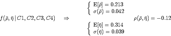
Expected values and standard deviations are obtained by numerical
integration. The result is
 |
 |
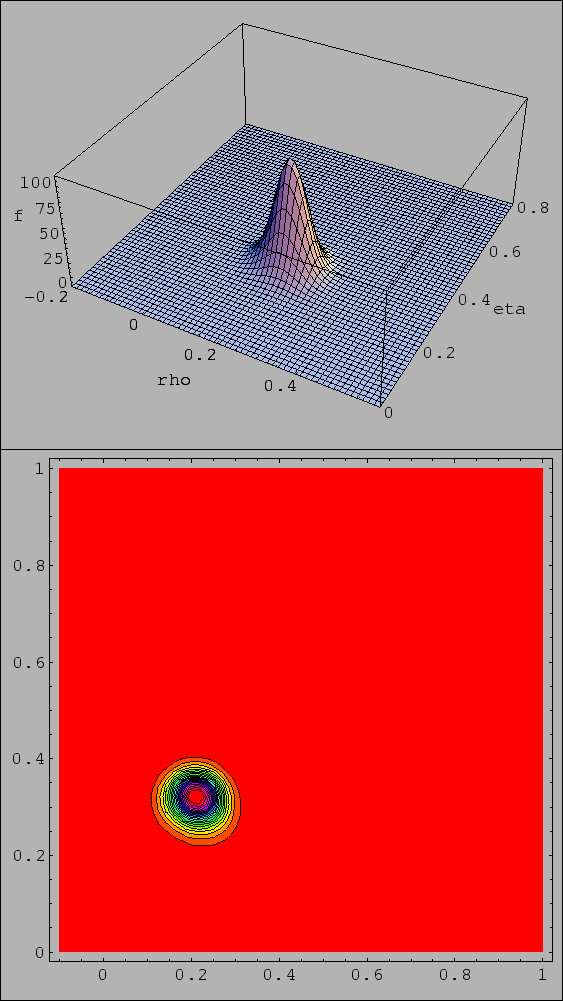
It is interesting to show partial and global results
as contour lines at ![]() of the maximum of the
reweighting functions, equivalent to the
of the maximum of the
reweighting functions, equivalent to the
![]() or
or
![]() rules2(I refer to Ref. [1] for the relation between
``standard'' methods based on
rules2(I refer to Ref. [1] for the relation between
``standard'' methods based on ![]() minimization
and the more detailed inferential scheme illustrated there).
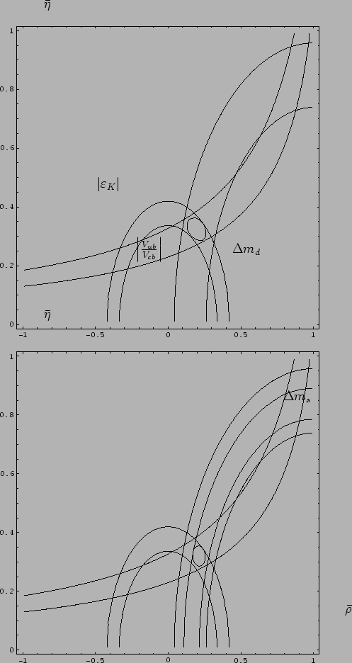
The top plot of Fig. 9 shows the contour
``roads''
given by the first three constraints, together with
the (almost) ellipse of their combination. The probability
that the values of
minimization
and the more detailed inferential scheme illustrated there).
The top plot of Fig. 9 shows the contour
``roads''
given by the first three constraints, together with
the (almost) ellipse of their combination. The probability
that the values of ![]() and
and ![]() are
both in the ellipse is about
37%.3
Instead, the projections of the ellipse on each axis gives
an interval of about
are
both in the ellipse is about
37%.3
Instead, the projections of the ellipse on each axis gives
an interval of about ![]() probability in each
variable.
probability in each
variable.
The bottom plot of Fig. 9 shows the effect
of the constraint ![]() . First we notice the perfect agreement
between the
. First we notice the perfect agreement
between the ![]() and
and ![]() roads, indicating that the
values of
roads, indicating that the
values of ![]() suggested by the data are absolutely
consistent with the other constraints within the Standard Model.
Furthermore, the effect of the
suggested by the data are absolutely
consistent with the other constraints within the Standard Model.
Furthermore, the effect of the ![]() on the ``ellipse'' of the
final inference is to reshape the left side, increasing the value
of
on the ``ellipse'' of the
final inference is to reshape the left side, increasing the value
of ![]() and decreasing its uncertainty, with almost no
effect on
and decreasing its uncertainty, with almost no
effect on ![]() , as also shown by the results (16)
and (17).
, as also shown by the results (16)
and (17).