Comparison of models of different complexity

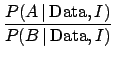
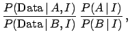
We have seen so far two typical inferential situations:

1. Comparison of simple models (Sect. 4), where by simple we mean that the models do not depend on parameters to be tuned to the experimental data.
2. Parametric inference given a model, to which we have devoted the last sections.

A more complex situation arises when we have several models, each of which might depend on several parameters. For simplicity, let us consider model $A$ with $n_A$ parameters ${\mbox{\boldmath$\alpha$}}$ and model $B$ with $n_B$ parameters ${\mbox{\boldmath$\beta$}}$. In principle, the same Bayesian reasoning seen previously holds:

$$\frac{P(A \,\vert\,\mbox{Data},I)}{P(B \,\vert\,\mbox{Data},I)} = \frac{P(\mbox{Data} \,\vert\,A,I)}{P(\mbox{Data} \,\vert\,B,I)}\, \frac{P(A \,\vert\,I)}{P(B \,\vert\,I)}\,,$$ (88)

but we have to remember that the probability of the data, given a model, depends on the probability of the data, given a model and any particular set of parameters, weighted with the prior beliefs about parameters. We can use the same decomposition formula (see Tab. 1), already applied in treating systematic errors (Sect. 6):

$$P(\mbox{Data} \,\vert\,M,I) = \int\!P(\mbox{Data} \,\vert\,M,{\mbox{\boldmath$\theta$}}, I) \,p({\mbox{\boldmath$\theta$}} \,\vert\,I)\,\mbox{d}{\mbox{\boldmath$\theta$}} \,,$$ (89)

with $M=A,B$ and ${\mbox{\boldmath$\theta$}} = {\mbox{\boldmath$\alpha$}}, {\mbox{\boldmath$\beta$}}$. In particular, the Bayes factor appearing in Eq. (88) becomes

$$\frac{P(\mbox{Data} \,\vert\,A,I)}{P(\mbox{Data} \,\vert\,B,I)} = \frac {\int\!P(\mbox{Data} \,\vert\,A,{\mbox{\boldmath$\alpha$}},... ...) \,p({\mbox{\boldmath$\beta$}} \,\vert\,I)\,\mbox{d}{\mbox{\boldmath$\beta$}}}$$ (90)

$$= \frac {\int\!{\cal L}_A({\mbox{\boldmath$\alpha$}};\, \mbox{Data}... ...Data}) \,p_0({\mbox{\boldmath$\beta$}}) \,\mbox{d}{\mbox{\boldmath$\beta$}}}\,.$$ (91)

The inference depends on the marginalized likelihood (89), also known as the evidence. Note that ${\cal L}_M({\mbox{\boldmath$\theta$}};\, \mbox{Data})$ has its largest value around the maximum likelihood point ${\mbox{\boldmath$\theta$}}_{ML}$, but the evidence takes into account all prior possibilities of the parameters. Thus, it is not enough that the best fit of one model is superior to its alternative, in the sense that, for instance,

$${\cal L}_A({\mbox{\boldmath$\alpha$}}_{ML};\, \mbox{Data}) > {\cal L}_B({\mbox{\boldmath$\beta$}}_{ML};\, \mbox{Data})\,,$$ (92)

and hence, assuming Gaussian models,

$$\chi^2_A({\mbox{\boldmath$\alpha$}}_{min\,\chi^2};\, \mbox{Data}) < \chi^2_B({\mbox{\boldmath$\beta$}}_{min\,\chi^2};\, \mbox{Data})\,,$$ (93)

to prefer model $A$. We have already seen that we need to take into account the prior beliefs in $A$ and $B$. But even this is not enough: we also need to consider the space of possibilities and then the adaptation capability of each model. It is well understood that we do not choose an $(n-1)$ order polynomial as the best description - `best' in inferential terms - of $n$ experimental points, though such a model always offers an exact pointwise fit. Similarly, we are much more impressed by, and we tend a posteriori to believe more in, a theory that absolutely predicts an experimental observation, within a reasonable error, than another theory that performs similarly or even better after having adjusted many parameters.

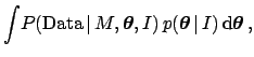
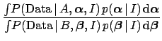
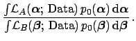
This intuitive reasoning is expressed formally in Eqs. (90) and (91). The evidence is given integrating the product ${\cal L}({\mbox{\boldmath$\theta$}})$ and $p_0({\mbox{\boldmath$\theta$}})$ over the parameter space. So, the more $p_0({\mbox{\boldmath$\theta$}})$ is concentrated around ${\mbox{\boldmath$\theta$}}_{ML}$, the greater is the evidence in favor of that model. Instead, a model with a volume of the parameter space much larger than the one selected by ${\cal L}({\mbox{\boldmath$\theta$}})$ gets disfavored. The extreme limit is that of a hypothetical model with so many parameters to describe whatever we shall observe. This effect is very welcome, and follows the Ockham's Razor scientific rule of discarding unnecessarily complicated models (``entities should not be multiplied unnecessarily''). This rule comes out of the Bayesian approach automatically and it is discussed, with examples of applications in many papers. Berger and Jefferys (1992) introduce the connection between Ockham's Razor and Bayesian reasoning, and discuss the evidence provided by the motion of Mercury's perihelion in favor of Einstein's general relativity theory, compared to alternatives at that time. Examples of recent applications are Loredo and Lamb 2002 (analysis of neutrinos observed from supernova SN 1987A), John and Narlikar 2002 (comparisons of cosmological models), Hobson et al 2002 (combination of cosmological datasets) and Astone et al 2003 (analysis of coincidence data from gravitational wave detectors). These papers also give a concise account of underlying Bayesian ideas.

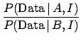
After having emphasized the merits of model comparison formalized in Eqs. (90) and (91), it is important to mention a related problem. In parametric inference we have seen that we can make an easy use of improper priors (see Tab. 1), seen as limits of proper priors, essentially because they simplify in the Bayes formula. For example, we considered $p_0(\mu \,\vert\,I)$ of Eq. (26) to be a constant, but this constant goes to zero as the range of $\mu$ diverges. Therefore, it does simplify in Eq. (26), but not, in general, in Eqs. (90) and (91), unless models $A$ and $B$ depend on the same number of parameters defined in the same ranges. Therefore, the general case of model comparison is limited to proper priors, and needs to be thought through better than when making parametric inference.