- ...
positive.1
- For examples of measurements
having
 and
and  with all combinations of
signs, see public online tables of Deep Inelastic
Scattering results.[1]
I want to make clear since the very beginning
that it is not my intention
to blame experimental or theoretical teams which have
reported in the past asymmetric uncertainty,
because we are all victims
of a bad tradition in data analysis. At least,
when asymmetric uncertainties have been given,
there is some chance to correct the result, as described in
Sec. 4. Since some asymmetric contributions to the
global uncertainties almost unavoidably happen in complex experiments,
I am more worried of collaborations that never
arrive to final asymmetric
uncertainties, because I must imagine they have
symmetrised somehow the result but, I am afraid, without
applying the proper shifts to the `best value' to take into account
asymmetric contributions, as it will be discussed in the present paper.
with all combinations of
signs, see public online tables of Deep Inelastic
Scattering results.[1]
I want to make clear since the very beginning
that it is not my intention
to blame experimental or theoretical teams which have
reported in the past asymmetric uncertainty,
because we are all victims
of a bad tradition in data analysis. At least,
when asymmetric uncertainties have been given,
there is some chance to correct the result, as described in
Sec. 4. Since some asymmetric contributions to the
global uncertainties almost unavoidably happen in complex experiments,
I am more worried of collaborations that never
arrive to final asymmetric
uncertainties, because I must imagine they have
symmetrised somehow the result but, I am afraid, without
applying the proper shifts to the `best value' to take into account
asymmetric contributions, as it will be discussed in the present paper.
.
.
.
.
.
.
.
.
.
.
.
.
.
.
.
.
.
.
.
.
.
.
.
.
.
.
.
.
.
.
- ... implicitly2
- Perhaps the reader would
be surprised to learn that in the conventional statistical
approach there is no room for probabilistic
statements about the value of physics quantities
(e.g.
``the top mass is between 170 and 180 GeV with
such percent probability'', or ``there is 95% probability that the
Higgs mass is lighter than 200 GeV''),
calibration constants, and so on, as discussed extensively
in Ref. [8].
.
.
.
.
.
.
.
.
.
.
.
.
.
.
.
.
.
.
.
.
.
.
.
.
.
.
.
.
.
.
- ...
results3
- The reader might be curious to know what would happen
in case of bad combinations of input
quantities with skewness of mixed signs.
Clearly there will be some compensation that lowers the risk of
strong bias. As an academic exercise, let think of five independent
variables each
described by the triangular distribution of Fig. 1
and five others each described by a p.d.f. which is its mirror reflexed
around
 [
[ ,
,
 ,
,
![$\mbox{E}[X] = 0.83$](img46.png) and
and
 ]. The correct combination of the ten variables
gives
]. The correct combination of the ten variables
gives
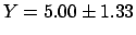 , while
adding the modes and combining quadratically left and right deviations
we would get
, while
adding the modes and combining quadratically left and right deviations
we would get  .
.
.
.
.
.
.
.
.
.
.
.
.
.
.
.
.
.
.
.
.
.
.
.
.
.
.
.
.
.
.
.
- ... function4
- But not yet a probability function!
The likelihood has the probabilistic meaning of a joined
p.d.f. of the data given
 ,
and not the other way around.
,
and not the other way around.
.
.
.
.
.
.
.
.
.
.
.
.
.
.
.
.
.
.
.
.
.
.
.
.
.
.
.
.
.
.
- ...
on.5
- has not a probabilistic
interpretation in the frequentistic approach,
and therefore we cannot
speak consistently, in that framework,
about its probability, or determine expectation,
standard deviation and so on. Most physicists do not even know
of this problem and think these are irrelevant semantic quibbles.
However, it is exactly this contradiction between intuitive thinking and
cultural background[8] that causes wrong
scientific conclusions, like those discussed in this paper.
.
.
.
.
.
.
.
.
.
.
.
.
.
.
.
.
.
.
.
.
.
.
.
.
.
.
.
.
.
.
- ... exception.6
- It is a matter of fact that
the habit in the particle physics community of applying uncritically
the
 or
or
 is related
to the use of the software package MINUIT[10].
Indeed, MINUIT can calculate the parameter variances
also from the
is related
to the use of the software package MINUIT[10].
Indeed, MINUIT can calculate the parameter variances
also from the  or
or  curvature at the minimum
(that relies on the same hypothesis
upon which the
or
rules are based). But when the or
are no longer parabolic, the standard deviation calculated from the
curvature
differs from that
of the
or
(in particular, when the minimized function is asymmetric
the latter rules give two values, the (in-)famous
curvature at the minimum
(that relies on the same hypothesis
upon which the
or
rules are based). But when the or
are no longer parabolic, the standard deviation calculated from the
curvature
differs from that
of the
or
(in particular, when the minimized function is asymmetric
the latter rules give two values, the (in-)famous  we are dealing with).
People realize
that the curvature at the minimum depends from the local behavior
of the minimized curve, and the
or
rule is typically more stable. Therefore, in particle physics
the latter rule has become de facto a standard to evaluate
`confidence intervals' at different `levels of confidence'
(depending of the value of the
we are dealing with).
People realize
that the curvature at the minimum depends from the local behavior
of the minimized curve, and the
or
rule is typically more stable. Therefore, in particle physics
the latter rule has become de facto a standard to evaluate
`confidence intervals' at different `levels of confidence'
(depending of the value of the  or
or
 ).
But, unfortunately, when those famous curves are not parabolic,
numbers obtained by these rules might loose completely a probabilistic meaning.
[Sorry, a frequentist would object that, indeed, these numbers do not
have probabilistic meaning about , but they are `confidence intervals'
at such and such `confidence level', because ` is
a constant of unknown value', etc...Good luck!]
).
But, unfortunately, when those famous curves are not parabolic,
numbers obtained by these rules might loose completely a probabilistic meaning.
[Sorry, a frequentist would object that, indeed, these numbers do not
have probabilistic meaning about , but they are `confidence intervals'
at such and such `confidence level', because ` is
a constant of unknown value', etc...Good luck!]
.
.
.
.
.
.
.
.
.
.
.
.
.
.
.
.
.
.
.
.
.
.
.
.
.
.
.
.
.
.
- ...
problem.7
- To be precise, this approximation
is valid if the parameters appear only in the argument of the exponent.
In practice this means that the fitted parameters must not appear in the
covariance matrix on which the depends.
As a simple example in which
this approximation do not hold is that of a linear fit in which
also the standard deviation
 describing the errors along the
ordinate. The joint inference about line coefficients
describing the errors along the
ordinate. The joint inference about line coefficients  and
and  and , having observed
  points,
is achieved by
points,
is achieved by
 (see Sec. 8.2 of Ref. [3]).
.
.
.
.
.
.
.
.
.
.
.
.
.
.
.
.
.
.
.
.
.
.
.
.
.
.
.
.
.
.
- ...
parameters.8
- See footnote 7 concerning a possible
pitfall in the use of
 .
.
.
.
.
.
.
.
.
.
.
.
.
.
.
.
.
.
.
.
.
.
.
.
.
.
.
.
.
.
.
.
- ...
numerically9
- Note that sometimes people do not get
asymmetric uncertainty, not because the propagation is
approximately linear,
but because asymmetry is hidden by the standard propagation
formula! Therefore also in this case the approximation might produce
a bias in the result (for example, the second order formula of the
expected value of the ratio of two quantities is known to
experts[12]). The merit of numerical derivatives
is that at least it shows the asymmetries.
.
.
.
.
.
.
.
.
.
.
.
.
.
.
.
.
.
.
.
.
.
.
.
.
.
.
.
.
.
.
- ...
deviations10
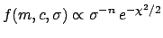
- In
terms of analytically calculated derivatives,
 and
and
 are given by
.
.
.
.
.
.
.
.
.
.
.
.
.
.
.
.
.
.
.
.
.
.
.
.
.
.
.
.
.
.
- ... variable.11
- After
what we have seen in Sec. 2
we should not forget that the input quantities could have non
trivial shapes. Since skewness and kurtosis are related to 3rd and 4th
moment of the distribution, Eq. (22)
makes use up to the 4th moment and is definitely better that
the usual propagation formula, that uses only second moments.
In Ref. [2] approximated formulae are given also
for skewness and kurtosis of the output variable,
from which it is possible to reconstruct
 taking into account
up to 4-th order moment of the distribution.
taking into account
up to 4-th order moment of the distribution.
.
.
.
.
.
.
.
.
.
.
.
.
.
.
.
.
.
.
.
.
.
.
.
.
.
.
.
.
.
.
- ...
attempts12
- It has been studied by psychologists how sometimes
our efforts to solve a problem are the analogous with the
moves along elements of a group structure (in the mathematical sense).
There is no way to reach a solution until we not
break out of this kind of trapping
psychological or cultural cages.[13]
.
.
.
.
.
.
.
.
.
.
.
.
.
.
.
.
.
.
.
.
.
.
.
.
.
.
.
.
.
.
- ... too.13
- In
this special case there should be
no doubt that a shift should be applied
to the best value, since moving
 by
by
 around its expected value
 ![$\mbox{E}[X_i]$](img147.png) the final quantity
the final quantity  only moves
in one side of
only moves
in one side of
![$Y(\mbox{E}[X_i])$](img148.png) .
.
.
.
.
.
.
.
.
.
.
.
.
.
.
.
.
.
.
.
.
.
.
.
.
.
.
.
.
.
.
.
- ...
become14
- The ISO Guide [14]
recommends to give the result using the standard
deviation within parenthesis, instead
of using the
 notation.
In this example we would have
notation.
In this example we would have
 .
Personally, I do not think this is
a very important issue as long as we know what the quantity
.
Personally, I do not think this is
a very important issue as long as we know what the quantity
 means. Anyhow, I understand the ISO rational,
and perhaps the proposed notation could help to make a break with
the `confidence intervals'.
means. Anyhow, I understand the ISO rational,
and perhaps the proposed notation could help to make a break with
the `confidence intervals'.
.
.
.
.
.
.
.
.
.
.
.
.
.
.
.
.
.
.
.
.
.
.
.
.
.
.
.
.
.
.
- ...eq:exact_corr_sigma).15
- The
slight difference between the standard deviations comes from
rounding, since
 of
Fig. 2 is the rounded value
of 1.54. Replacing 1.5 by 1.54 in Eq. (38),
we get exactly the Monte Carlo value of 1.65.
of
Fig. 2 is the rounded value
of 1.54. Replacing 1.5 by 1.54 in Eq. (38),
we get exactly the Monte Carlo value of 1.65.
.
.
.
.
.
.
.
.
.
.
.
.
.
.
.
.
.
.
.
.
.
.
.
.
.
.
.
.
.
.
- ... uncertainties16
- Discussing this issues with several
persons I have realized, with my great surprise, that this
misconception is deeply rooted and strenuously defended by many colleagues,
even by data analysis experts
(they constantly reply ``yes, but...'').
This attitude is probably one of the consequences of being
anchored to what I call un-needed principles
(namely maximum likelihood, in this case), such
that even the digits resulting from these
principles are taken with a kind of religious respect
and it seems blasphemous to touch them.
.
.
.
.
.
.
.
.
.
.
.
.
.
.
.
.
.
.
.
.
.
.
.
.
.
.
.
.
.
.
- ... intervals,17
- I give
the central 68.3% interval with some reluctance,
because I know by experience that in many minds
the short circuit
is almost unavoidable (I have known physicists convinced
- and who even taught it! -
that the standard deviation only `makes sense for the Gaussian'
and that it was defined via the `68% rule'). For this
reason, recently I have started to appreciate thinking in terms of
50% probability intervals, also because they force people to reason
in terms of better perceived
fifty-to-fifty bets. I find these kind of bets very enlighting
to show why practically all standard ways (including Bayesian ones!)
fail to report upper/lower
confidence limits in frontier case situations characterized
by open likelihoods (see chapter 12 in Ref.[3]). I like to ask
``please use your method and give me a 50% C.L. upper/lower limit'',
and then, when I have got it,
``are you really 50% confident that the value is below
that limit and 50% confident that it is above it?
Would you equally bet on either side of that limit?''.
And the supporters of `objective' methods
are immediately at loss. (At least those who use Bayesian formulae
realize that there must be some problem with the choice
of priors.)
.
.
.
.
.
.
.
.
.
.
.
.
.
.
.
.
.
.
.
.
.
.
.
.
.
.
.
.
.
.
- ... case18
- In the example here
we have been lucky because an over-correction
of the first contribution was compensated by an under-correction
of the second contribution. Note also that the hypothesis
about the nonlinear propagation was not correct, because we had,
instead, a linear propagation of asymmetric p.d.f.'s. Anyhow
the overall shift calculated by the guessed hypothesis
is comparable to that calculable knowing the details of the analysis
(and, in any case, using in subsequent analyses
the roughly corrected result is
definitely better than sticking to the published `best value').
.
.
.
.
.
.
.
.
.
.
.
.
.
.
.
.
.
.
.
.
.
.
.
.
.
.
.
.
.
.
- ...
result.19
- Note that even if we were told that was
 , without further information, we could
still try to apply some shift to the result, obtaining
, without further information, we could
still try to apply some shift to the result, obtaining
 or
or  depending on some guesses
about the source of the asymmetry. In any case, either
results are better than
!
depending on some guesses
about the source of the asymmetry. In any case, either
results are better than
!
.
.
.
.
.
.
.
.
.
.
.
.
.
.
.
.
.
.
.
.
.
.
.
.
.
.
.
.
.
.
![$\displaystyle \frac{1}{2}\left.\frac{\partial^2 Y}
{\partial X^2}\right\vert _{\mbox{\small E}[X]}
\sigma^2(X)$](img124.png)
![$\displaystyle \left.\frac{\partial Y}
{\partial X}\right\vert _{\mbox{\small E}[X]}
\sigma(X) .$](img126.png)