Nonlinear propagation

Another source of asymmetric uncertainties is nonlinear dependence of the output quantity $Y$ on some of the input ${\mbox{\boldmath$X$}}$ in a region a few standard deviations around $\mbox{E}({\mbox{\boldmath$X$}})$. This problem has been studied with great detail in Ref. [2], also taking into account correlations on input and output quantities, and somewhat summarized in Ref. [3]. Let us recall here only the most relevant outcomes, in the simplest case of only one output quantity $Y$ and neglecting correlations.

Figure: Propagation of a Gaussian distribution under a nonlinear transformation. $f(Y_i)$ were obtained analytically using Eq.(1) (part of Fig. 12.2 of Ref.[3]).

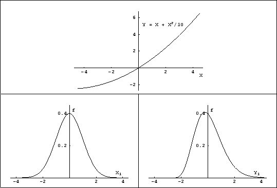Figure 4 shows a non linear dependence between $X$ and $Y$ and how a Gaussian distribution has been distorted by the transformation [$f(y)$ has been evaluated analytically using Eq.(1)]. As a result of the nonlinear transformation, mode, mean, median and standard deviation are transformed in non trivial ways (in the example of Fig. 4 mode moves left and expected value right). In the general case the complete calculations should be performed, either analytically, or numerically or by Monte Carlo. Fortunately, as it has been shown in Ref. [2], second order expansion is often enough to take into account small deviations from linearity. The resulting formulae are still compact and depend on location and shape parameters of the initial distributions.

Second order propagation formulae depend on first and second derivatives. In practical cases (especially as far as the contribution from systematic effects are concerned) the derivatives are obtained numerically⁹ as

$$\left.\frac{\partial Y}{\partial X}\right\vert _{\mbox{\small E}[X]} \approx \frac{1}{2} \left(\frac{\Delta _+}{\sigma(X)}+ \frac{\Delta _-}{\sigma(X)}\right) = \frac{\Delta _+ +\Delta _-}{2 \sigma(X)} ,$$ (17)

$$\left.\frac{\partial^2 Y}{\partial X^2}\right\vert _{\mbox{\small E}[X]} \approx \frac{1}{\sigma(X)} \left(\frac{\Delta _+}{\sigma(X)}-\frac{\Delta _-}{\sigma(X)}\right) = \frac{\Delta _+-\Delta _-}{\sigma^2(X)} ,$$ (18)

where $\Delta_-$ and $\Delta_+$ now stand for the left and right deviations of $Y$ when the input variable $X$ varies by one standard deviation around $\mbox{E}[X]$. Second order propagation formulae are conveniently given in Ref. [2] in terms of the $\Delta_\pm$ deviations¹⁰. For $Y$ that depends only on a single input $X$ we get:

$$\mbox{E}(Y) \approx Y(\mbox{E}[X]) + \delta ,$$ (21)

$$\sigma^2(Y) \approx \overline{\Delta}^2 + 2 \overline{\Delta}\cdot\delta\cdot S(X)+ \delta^2\cdot\left[{\cal K}(X)-1\right] ,$$ (22)

where $\delta$ is the semi-difference of the two deviations and $\overline{\Delta}$ is their average:

$$\delta = \frac{\Delta _{+}-\Delta _{-}}{2}$$ (23)

$$\overline{\Delta} = \frac{\Delta _{+}+\Delta _{-}}{2} ,$$ (24)

while ${\cal S}(X)$ and ${\cal K}(X)$ stand for skewness and kurtosis of the input variable.¹¹

For many input quantities we have

$$\mbox{E}(Y) \approx Y(\mbox{E}[X]) + \sum_i\delta_i ,$$ (25)

$$\sigma^2(Y) \approx \sum_i\sigma^2_{X_i}(Y) ,$$ (26)

where $\sigma^2_{X_i}(Y)$ stands for each individual contribution to Eq. (22). The expression of the variance gets simplified when all input quantities are Gaussian (a Gaussian has skewness equal 0 and kurtosis equal 3):

$$\sigma^2(Y) \approx \sum_i\overline{\Delta}^2_i+2\sum_i \delta^2_i ,$$ (27)

and, as long as $\delta_i^2$ are much smaller that $\overline{\Delta}_i^2$, we get the convenient approximated formulae

$$\mbox{E}(Y) \approx Y(\mbox{E}[{{\mbox{\boldmath$X$}}}]) + \sum_i \delta_i ,$$ (28)

$$\sigma^2(Y) \approx \sum_i \overline{\Delta}^2_i$$ (29)

valid also for other symmetric input p.d.f.'s (the kurtosis is about 2 to 3 in typical distribution and its exact value is irrelevant if the condition 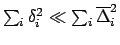$\sum_i\delta_i^2 \ll \sum_i\overline{\Delta}_i^2$ holds). The resulting practical rules (28)-(29) are quite simple:

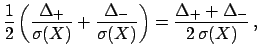
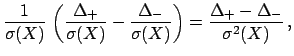
• the expected value of $Y$ is shifted by the sum of the individual shifts, each given by half of the semi-difference of the deviations $\Delta_\pm$;
• each input quantity contributes (in quadrature) to the combined standard uncertainty with a term which is approximately the average between the deviations $\Delta_\pm$.

Moreover, if there are many contributions to the uncertainty, the final uncertainty will be symmetric and approximately Gaussian, thanks to the central limit theorem.