


Next: Nonlinear propagation
Up: Sources of asymmetric uncertainties
Previous: Sources of asymmetric uncertainties
The standard methods in physics to adjust theoretical parameters to
experimental data are based on maximum likelihood principle
ideas.
In practice, depending on the situation, the `minus log-likelihood'
of the parameters
[
 ]
or the
]
or the  function of the parameters [i.e. the function
 ] are minimized.
The notation used reminds
that
] are minimized.
The notation used reminds
that  and are seen as
mathematical function of the parameters
and are seen as
mathematical function of the parameters
 , with the data acting as `parameters' of the functions.
As it is well understood, a part from an irrelevant constant non
depending on fit parameters,
and differ by just a factor of two
when the likelihood, seen as a joint probability function or a p.d.f.
of the data,
is a (multivariate) Gaussian distribution of the data:
, with the data acting as `parameters' of the functions.
As it is well understood, a part from an irrelevant constant non
depending on fit parameters,
and differ by just a factor of two
when the likelihood, seen as a joint probability function or a p.d.f.
of the data,
is a (multivariate) Gaussian distribution of the data:
 (the constant
  is often neglected,
since we concentrate on the terms which depend on the fit
parameters - but sometimes and minus log-likelihood
might differ by terms depending on fit parameters!).
For sake of simplicity, let us take one parameter fit.
Following the usual practice, we indicate the parameter by
is often neglected,
since we concentrate on the terms which depend on the fit
parameters - but sometimes and minus log-likelihood
might differ by terms depending on fit parameters!).
For sake of simplicity, let us take one parameter fit.
Following the usual practice, we indicate the parameter by  (though this fit parameter is just any of the input quantities
 of Sec. 2).
If
 or
or
 have a nice parabolic
shape,
the likelihood is, apart a multiplicative factor,
a Gaussian function4 of .
In fact, as is well known from calculus,
any function can be approximated to a parabola in the vicinity
of its minimum.
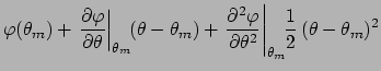
Let us see in detail the expansion of
around its minimum
have a nice parabolic
shape,
the likelihood is, apart a multiplicative factor,
a Gaussian function4 of .
In fact, as is well known from calculus,
any function can be approximated to a parabola in the vicinity
of its minimum.
Let us see in detail the expansion of
around its minimum
 :
:
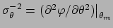
where the second term of the r.h.s. vanishes by definition
of minimum and we have indicated with  the
inverse of the second derivative at the minimum.
Going back to the likelihood, we get:
the
inverse of the second derivative at the minimum.
Going back to the likelihood, we get:
apart a multiplicative factor, this is
`Gaussian'
centered in
with standard deviation
 .
However, although this function is mathematically
a Gaussian, it does not have yet the meaning of
probability density
.
However, although this function is mathematically
a Gaussian, it does not have yet the meaning of
probability density
 in an inferential
sense, i.e. describing our knowledge about in the light
of the experimental data. In order to do this, we need to process
the likelihood through Bayes theorem,
which allows probabilistic inversions to be achieved using
basic rules of probability theory and logic.
Besides a conceptually irrelevant normalization factor
(that has to be calculated at some moment) the Bayes formula is
in an inferential
sense, i.e. describing our knowledge about in the light
of the experimental data. In order to do this, we need to process
the likelihood through Bayes theorem,
which allows probabilistic inversions to be achieved using
basic rules of probability theory and logic.
Besides a conceptually irrelevant normalization factor
(that has to be calculated at some moment) the Bayes formula is
We can speak now about the ``probability that is
within a given interval'' and calculate it, together
with expectation of , standard deviation
and so
on.5
If the prior  is much
vaguer that what the
data can teach us (via the likelihood),
then it can be re-absorbed in the normalization constant,
and we get:
is much
vaguer that what the
data can teach us (via the likelihood),
then it can be re-absorbed in the normalization constant,
and we get:
If this is the case, it is a simple exercise to show that
- a)
-
![$\mbox{E}[\theta]$](img85.png) is equal to which minimizes the
or .
is equal to which minimizes the
or .
- b)
 can be obtained by the famous conditions
 or
or
 , respectively,
or by the second derivative around :
, respectively,
or by the second derivative around :
 or
or
 ,
respectively.
,
respectively.
Though in the frequentistic approach language and methods are usually
more convoluted (even when the same numerical results of the Bayesian
reasoning are obtained), due to the fact that probabilistic statements
about physics quantities and fit parameters are not
allowed in that approach, it is usually accepted that
the above rules  and
and  are based on the parabolic behavior of
the minimized functions.
When this approximation does not hold, the
frequentist has to replace a prescription by other prescriptions
that can handle the exception.6
The situation is simpler and clearer
in the Bayesian approach, in which the above rules and do hold too,
but only as approximations under well defined conditions.
In case the underlying conditions fail
we know immediately what to do:
are based on the parabolic behavior of
the minimized functions.
When this approximation does not hold, the
frequentist has to replace a prescription by other prescriptions
that can handle the exception.6
The situation is simpler and clearer
in the Bayesian approach, in which the above rules and do hold too,
but only as approximations under well defined conditions.
In case the underlying conditions fail
we know immediately what to do:
- restart from Eq. (9) or from Eq. (11),
depending on the other underlying hypotheses;
- go even one step before Eq. (9),
namely to the most general Eq. (8),
if priors matter
(e.g. physical constraints, sensible previous knowledge, etc.).
For example, if the description of the data was a
good approximation,
then
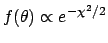 ,
properly normalized, is the solution to the
problem.7
,
properly normalized, is the solution to the
problem.7
Figure:
Example (Ref. [3]) of asymmetric curve
(left plot)
with a minimum at  (
( stands for the value
of a generic physics quantity).
The result based on the
stands for the value
of a generic physics quantity).
The result based on the
 `prescription'
is compared (plot on the right side)
with the p.d.f. based
on a uniform prior, i.e.
`prescription'
is compared (plot on the right side)
with the p.d.f. based
on a uniform prior, i.e.
![$f(\mu \vert \mbox{data})\propto \exp[-\chi^2/2]$](img102.png) .
.
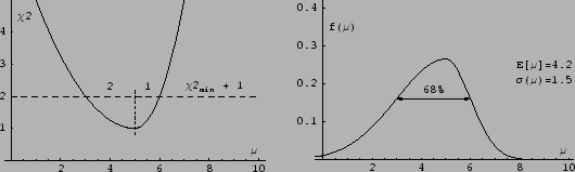 |
A non parabolic, asymmetric produces an asymmetric
 (see Fig. 2),
the mode of which corresponds, indeed, to what obtained
minimizing , but expected value and standard deviation
differ from what is obtained by the `standard rule'.
In particular, expected value and variance must be
evaluated from their definitions:
(see Fig. 2),
the mode of which corresponds, indeed, to what obtained
minimizing , but expected value and standard deviation
differ from what is obtained by the `standard rule'.
In particular, expected value and variance must be
evaluated from their definitions:
Other examples of asymmetric curves, including the case
with more than one minimum, are shown in Chapter 12 of Ref. [3],
and compared with the
results coming from frequentist prescriptions
(but, indeed, there is not a general accepted rule to
get frequentistic results - whatever they mean -
when the shape gets complicated).
Unfortunately,
it is not easy to translate numbers obtained by ad hoc
rules into probabilistic results, because the dependence
on the actual shape of the or curve can be
not trivial.
Anyhow,
some rules of thumb can be given in next-to-simple situations
where the or has only one minimum and
the or curve looks like a `skewed parabola',
like in Fig. 2:
Figure:
Example of two-dimensional multi-spots
``68% CL'' and ``95% CL'' contours obtained slicing
the
or the minus log-likelihood curve at some
magic levels. What do they mean?
 |
The remarks about misuse of
and
rules
can be extended to cases where several parameters are involved.
I do not want to go into details
(in the Bayesian approach there is
nothing deeper than studying
 or
or
 in function of several
parameters.8), but I just want
to get the reader
worried about the meaning of contour plots of the kind shown
in Fig. 3.
in function of several
parameters.8), but I just want
to get the reader
worried about the meaning of contour plots of the kind shown
in Fig. 3.
Next: Nonlinear propagation
Up: Sources of asymmetric uncertainties
Previous: Sources of asymmetric uncertainties
Giulio D'Agostini
2004-04-27
![$\displaystyle \exp{\left[- \varphi(\theta_m)\right]} \cdot
\exp{\left[-\frac{1}{2} \frac{1}{\alpha^2} (\theta-\theta_m)^2\right]}$](img68.png)
![$\displaystyle k \exp{\left[-\frac{(\theta-\theta_m)^2}
{2 \alpha^2}\right]} ,$](img69.png)
![$\displaystyle \exp{\left[-\frac{\chi^2(\theta;\mbox{data})}{2}\right]}$](img80.png)
![$\displaystyle \frac{1}{\sqrt{2\pi} \sigma_\theta}
\exp{\left[-\frac{(\theta-\mbox{\small E}[\theta])^2}
{2 \sigma_\theta^2}\right]} .$](img84.png)
![$\displaystyle \int\!(\theta-\mbox{E}[\theta])^2
f(\theta \vert \mbox{data}) \mbox{d}\theta .$](img108.png)