Propagating uncertainty

Determining the value of a physics quantity is seldom an end in itself. In most cases the result is used, together with other experimental and theoretical quantities, to calculate the value of other quantities of interest. As it is well understood, uncertainty on the value of each ingredient is propagated into uncertainty on the final result.

If uncertainty is quantified by probability, as it is commonly done explicitly or implicitly² in physics, the propagation of uncertainty is performed using rules based on probability theory. If we indicate by ${\mbox{\boldmath$X$}}$ the set (`vector') of input quantities and by $Y$ the final quantity, given by the function $Y=Y({\mbox{\boldmath$X$}})$ of the input quantities, the most general propagation formula (see e.g. [3]) is given by (we stick to continuous variables):

$$f(y) = \int\! \delta[y-Y({\mbox{\boldmath$x$}})]\cdot f({\mbox{\boldmath$x$}}) \mbox{d}{\mbox{\boldmath$x$}} ,$$ (1)

where $f(y)$ is the p.d.f. of $Y$, $f({\mbox{\boldmath$x$}})$ stands for the joint p.d.f. of ${\mbox{\boldmath$X$}}$ and $\delta$ is the Dirac delta (note the use of capital letters to name variables and small letters to indicate the values that variables may assume). The exact evaluation of Eq. (1) is often challenging, but, as discussed in Ref. [3], this formula has a nice simple interpretation that makes its Monte Carlo implementation conceptually easy.

As it is also well known, often there is no need to go through the analytic, numerical or Monte Carlo evaluation of Eq.(1), since linearization of $Y({\mbox{\boldmath$x$}})$ around the expected value of ${\mbox{\boldmath$X$}}$ (E[ ${\mbox{\boldmath$X$}}$]) makes the calculation of expected value and variance of $Y$ very easy, using the well known standard propagation formulae, that for uncorrelated input quantities are

$$\mbox{E}[Y] \approx Y(\mbox{E}[{\mbox{\boldmath$X$}}])$$ (2)

$$\sigma^2(Y) \approx \sum_i \left(\left.\frac{\partial Y}{\partial X_i} \right\vert _{\mbox{E}[{\mbox{\boldmath$X$}}]}\right)^2 \sigma^2(X_i) .$$ (3)

As far as the shape of $f(y)$, a Gaussian one is usually assumed, as a result of the central limit theorem. Holding this assumptions, $\mbox{E}[Y]$ and $\sigma(Y)$ is all what we need. $\mbox{E}[Y]$ gives the `best value', and probability intervals, upper/lower limits and so on can be easily calculated. In particular, within the Gaussian approximation, the most believable value (mode), the barycenter of the p.d.f. (expected value) and the value that separates two adjacent 50% probability intervals (median) coincide. If $f(y)$ is asymmetric this is not any longer true and one needs then to clarify what `best value' means, which could be one of the above three position parameters, or something else (in the Bayesian approach `best value' stands for expected value, unless differently specified).

Anyhow, Gaussian approximation is not the main issue here and, in most real applications, characterized by several contributions to the combined uncertainty about $Y$, this approximation is a reasonable one, even when some of the input quantities individually contribute asymmetrically. My concerns in this paper are more related to the evaluation of $\mbox{E}[Y]$ and $\sigma(Y)$ when

1. instead of Eqs. (2)-(3), ad hoc propagation prescriptions are used in presence of asymmetric uncertainties;
2. linearization implicit in Eqs. (2)-(3) is not a good approximation.

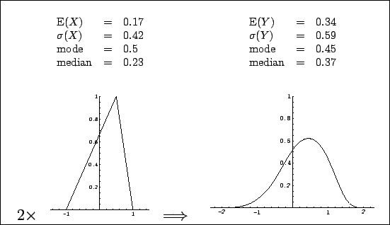
Let us start with the first point, considering, as an easy academic example, input quantities described by the asymmetric triangular distribution shown in the left plot of Fig. 1.

Figure: Distribution of the sum of two independent quantities, each described by an asymmetric triangular p.d.f. self-defined in the left plot. The resulting p.d.f. (right plot) has been calculated analytically making use of Eq.(1). This figure corresponds to Fig. 4.3 of Ref. [3].

The value of $X$ can range between $-1$ and $1$, with a `best value', in the sense of maximum probability value, of 0.5. The interval $[-0.16, +0.72]$ gives a 68.3% probability interval, and the `result' could be reported as $X_1=0.50^{+0.22}_{-0.66}$. This is not a problem as long as we known what this notation means and, possibly, know the shape of $f(x)$. The problem arises when we want to make use of this result and we do not have access to $f(x)$ (as it is often the case), or we make improper use of the information [i.e. in the case we are aware of $f(x)$]. Let us assume, for simplicity, to have a second independent quantity, $X_2$, described exactly by the same p.d.f. and reported in the same way: $X_2=0.50^{+0.22}_{-0.66}$. Imagine we are now interested to the quantity $Y=X_1+X_2$. How to report the result about $Y$, based on the results about $Y_1$ and $Y_2$? Here are some common, but wrong ways to give the result:

• asymmetric uncertainties added in quadrature: $Y=1.00^{+0.31}_{-0.93}$;
• asymmetric uncertainties added linearly: $Y=1.00^{+0.44}_{-1.31}$.

Indeed, in this simple case we can calculate the integral (1) analytically, obtaining the curve shown in the plot on the right side of Fig. 1, where several position and shape parameters have also been reported. The `best value' of $Y$, meant as expected value (i.e. the barycenter of the p.d.f.) comes out to be 0.34. Even those who like to think at the `best value' as the value of maximum probability (density) would choose 0.45 (note that in this particular example the mode of the sum is smaller than the mode of each addend!). Instead, a `best value' of $Y$ of 1.00 obtained by the ad hoc rules, unfortunately often used in physics, corresponds neither to mode, nor to expected value or median.

The situation would have been much better if expected value and standard deviation of $X_1$ and $X_2$ had been reported (respectively 0.17 and 0.42). Indeed, these are the quantities that matter in `error propagation', because the theorems upon which propagation formulae rely -- exactly in the case $Y$ is a linear combination of ${\mbox{\boldmath$X$}}$, or approximately in the case linearization has been performed -- speak of expected values and variances. It is easy to verify from the numbers in Fig. 1 that exactly the correct values of $\mbox{E}[Y] = 0.34$ and $\sigma(Y)=0.59$ would have been obtained. Moreover, one can see that expected value, mode and median of $f(y)$ do not differ much from each other, and the shape of $f(y)$ resembles a somewhat skewed Gaussian. When $Y$ will be combined with other quantities in a next analysis its slightly non-Gaussian shape will not matter any longer. Note that we have achieved this nice result already with only two input quantities. If we had a few more, already $Y$ would have been much Gaussian-like. Instead, performing a bad combination of several quantities all skewed in the same side would yield `divergent' results³: for $n=10$ we get, using a quadratic combination of left and right deviations, $Y=5.00^{+0.69}_{-2.07}$ versus the correct $Y=1.70\pm 1.32$.

As conclusion from this section I would like to make some points:

• in case of asymmetric uncertainty on a quantity, it should be avoided to report only most probable value and a probability interval (be it 68.3%, 95%, or what else);
• expected value, meant as barycenter of the distribution, as well as standard deviations should always be reported, providing also the shape of the distribution (or its summary in terms of shape parameters, or even a parameterization of the log-likelihood function in a polynomial form, as done e.g. in Ref. [9]), if the distribution is asymmetric or non trivial.

Note that the propagation example shown here is the most elementary possible. The situation gets more complicate if also nonlinear propagation is involved (see Sec. 3.2) or when quantities are used in fits (see e.g. Sec. 12.1 of Ref. [3]).

Hoping that the reader is, at this point, at least worried about the effects of badly treated asymmetric uncertainties, let us now review the sources of asymmetric uncertainties.