Importance sampling

In this method, too, we start from an `easy' function $g({\mbox{\boldmath$x$}})$, which `we hope' will approximate $p({\mbox{\boldmath$x$}})$ of interest, of which in fact we know only its un-normalized expression $\tilde p({\mbox{\boldmath$x$}})$. However, there is no requirement about how $g({\mbox{\boldmath$x$}})$ approximates $p({\mbox{\boldmath$x$}})$ (but the goodness of approximation will have an impact on the efficacy of the method), apart from the condition that $g({\mbox{\boldmath$x$}}_i)$ must be positive wherever $p({\mbox{\boldmath$x$}}_i)$ is positive .

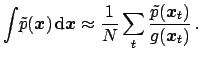
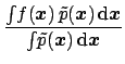
The function $g({\mbox{\boldmath$x$}})$ can be used in the calculation of $\mbox{E}[f({\mbox{\boldmath$x$}})]$, if we notice that $\mbox{E}[f({\mbox{\boldmath$x$}})]$ can be rewritten as follows:

$$\mbox{E}[f({\mbox{\boldmath$x$}})] = \frac{\int\! f({\mbox{\boldmath$x$}}) \, \tilde p({\mbox{\boldmat... ...h$x$}}} {\int\! \tilde p({\mbox{\boldmath$x$}})\,\mbox{d}{\mbox{\boldmath$x$}}}$$ (112)

$$= \frac{\int\! f({\mbox{\boldmath$x$}}) \, \left[\tilde p({\mbox{\b... ...oldmath$x$}})\right]\,g({\mbox{\boldmath$x$}}) \,\mbox{d}{\mbox{\boldmath$x$}}}$$ (113)

$$= \frac{\mbox{E}_g\left[ f({\mbox{\boldmath$x$}}) \, \tilde p({\mbo... ...x{E}_g\left[\tilde p({\mbox{\boldmath$x$}})/g({\mbox{\boldmath$x$}})\right]}\,,$$ (114)

where the the symbol $\mbox{E}_g$ is a reminder that the expectation is calculated over the distribution $g({\mbox{\boldmath$x$}})$. Finally, the strategy can be implemented in the Monte Carlo using Eq. (111) for the two expectations:

$$\mbox{E}[f({\mbox{\boldmath$x$}})] \approx \frac{ \sum_t f({\mbox{\boldmath$x$}}_t) \, \tilde p({\mbox{\bold... ..._t)} { \sum_t \tilde p({\mbox{\boldmath$x$}}_t)/g({\mbox{\boldmath$x$}}_t) }\,.$$ (115)

From the same sample it is also possible to evaluate the normalization constant, given by the denominator of Eq. (113), i.e.

$$Z = \int\! \tilde p({\mbox{\boldmath$x$}})\,\mbox{d}{\mbox{\boldmath$... ... \sum_t \frac{\tilde p({\mbox{\boldmath$x$}}_t)}{g({\mbox{\boldmath$x$}}_t)}\,.$$ (116)

The computation of this quantity is particularly important when we are dealing with model comparison and $Z$ has the meaning of `evidence' (Sect. 7).

It easily to see that the method works well if $g({\mbox{\boldmath$x$}})$ overlaps well with $p({\mbox{\boldmath$x$}})$. Thus, a proper choice of $g({\mbox{\boldmath$x$}})$ can be made by studying where the probability mass of $p({\mbox{\boldmath$x$}})$ is concentrated (for example finding the mode of the distribution in a numerical way). Often a Gaussian function is used for $g({\mbox{\boldmath$x$}})$, with parameters chosen to approximate $p({\mbox{\boldmath$x$}})$ in the proximity of the mode, as described in Sect. 5.10. In other cases, other functions can be used which have more pronounced tails, like $t$-Student or Cauchy distributions. Special techniques, into which we cannot enter here, allow $n$ independent random numbers to be generated and, subsequently, by proper rotations, turned into other numbers which have a correlation matrix equal to that of the multi-dimensional Gaussian which approximates $p({\mbox{\boldmath$x$}})$.

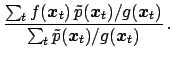
Note, finally, that, contrary to the rejection sampling, importance sampling is not suitable for generate samples of `unweighted events', such as those routinely used in the planning and the analysis of many kind experiments, especially particle physics experiments.