Sceptical analysis using the individual values of Ref. [8]

Let us know go into the details of the results which contribute to 5-th entry of Tab. 1, reported in Fig. 12 [8] and in the entries 5-8 of Tab. 2.

Table: Details of the individual result used in the overall analysis.

	Authors	pub. year	$[d_i]$	$[s_i]$
$i$			(MeV)	(MeV)
$1$	G. Backenstoss et al. [4]	1973	493.691	0.040
$2$	S.C. Cheng et al. [5]	1975	493.657	0.020
$3$	L.M. Barkov et al.[6]	1979	493.670	0.029
$4$	G.K. Lum et al. [7]	1981	493.640	0.054
$5$	K.P. Gall et al. [8]	1988	493.675	0.026
$6$			493.631	0.007
$7$			493.806	0.095
$8$			493.709	0.073
$9$	A.S. Denisov et al. & Yu.M. Ivanov [9,10]	1991	493.696	0.007

Figure: Standard and sceptical combination of the four data points of Ref. [8]. The dashed line is the simple weighted average; the gray line having the same center and larger width is the same with the standard deviation scaled by $\sqrt {\chi ^2/\nu }$ as done in Ref. [8]. The thick, asymmetric curve represent the result of the sceptical combination.

There is one high precision value favoring a small mass value ( $493.631\pm 0.007\,$MeV), and three values of minor precision preferring higher mass values. The simple weighted average of $493.6355\pm 0.0067\,$MeV is then practically equal to the highest precision value. But then a $\times 1.52$ scaling is applied by the authors. The combined uncertainty grows up, which is something desirable, but it does it symmetrically around the mean, not taking into account the fact that the other results would pull the mass value up.

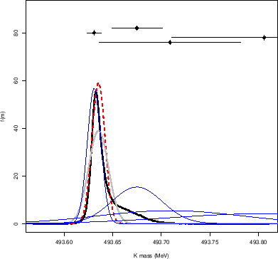It is then interesting to make a sceptical combination of these four points. The result is shown if Fig. 14. The sceptical analysis takes into account also the results favoring higher mass values, although the peak of the distribution (the `mode') remains very close to the most precise result, and there is a substantial overlap with it. The distribution is now skewed on the right side, assigning higher probability that the mass value is, for example, above $493.65\,$MeV with respect to what we could think judging from mean and standard deviation alone. The resulting mass is $493.642\pm 0.016\,$MeV shifted up by about $6\,$keV, with a standard uncertainty about 50% larger than that provided by the $\sqrt {\chi ^2/\nu }$ scaling prescription. But what is more interesting is that the latter (gray line in the figure, just below the red dashed one) does not give a correct account of the possible values of $m_{K^\pm}$, because: i) it is extended to the low mass values sizable more than the measured points would allow it; ii) it gives practically no chance to mass values above e.g. $493.657\,$MeV.

Finally there is the question of combining this result with the other five ones of other experiments. What should we use as input for the global analysis? Honestly, at this point we cannot pretend to have not seen the outcome shown in Fig. 14 and to use just the resulting average and standard uncertainty. We also cannot feed into the model the complicated posterior we have got. Therefore the only solution is to make a new combined analysis, but using all individual results of Ref. [8]. For sake of clarity all points are repeated in Tab. 2.

Figure: Combined analysis obtained considering the individual points of [8]. The not trivial final pdf of the sceptical analysis (thick continuous black line) can be summarized as $493.677\pm 0.013\,$MeV. The weighed average (dashed red) leads instead $493.6644\pm 0.0046$, which becomes $493.664\pm 0.011$ (solid gray Gaussian just below the dashed red one) when the standard deviation is scaled by the factor $\sqrt {\chi ^2/\nu } = \sqrt {47.7/8} = 2.42$.

The result of the analysis, plotted in Fig 15, is quite surprising on a first sight: while the standard weighted average is practically the same of Fig. 13 (small differences might be attributed to rounding²³), the sceptical combination moves up, disfavoring the low mass solution and yielding $493.677\pm 0.013\,$MeV.

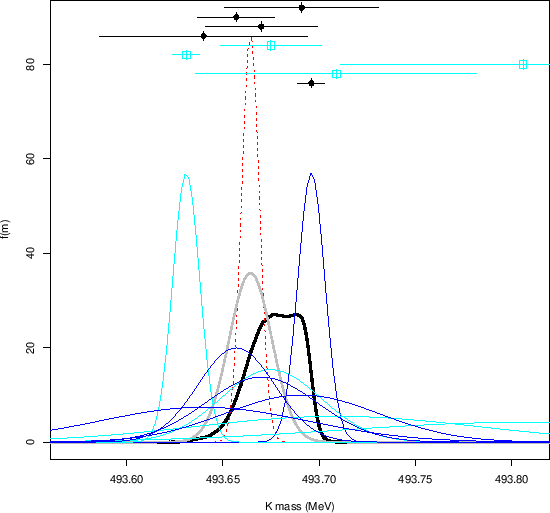“The same as the PDG result”, one would promptly shout at this point, “and after so much work!”. Well, yes and no... Indeed, the PDG numbers were obtained considering an arbitrarily enlarged uncertainty for the combined result of Ref. [8]. Applying, instead, the scaling prescription to the nine individual points of Tab. 2 a value of $493.664\pm 0.011\,$ MeV would have been obtained, $13\,$keV below the result of the sceptical analysis (see Fig.15). Certainly this $\approx - 1\,\sigma$ bias will not harm our understating of fundamental physics, but it is better to avoid this kind of biases because they could perhaps be important in other measurements.