- ... balls.
![[*]](footnote.png)
- Those who understand
Italian might form an idea of a real session watching
a video of a conference for the general public organized by
the University of Roma 3 in June 2016
(http://orientamento.matfis.uniroma3.it/fisincittastorico.php#dagostini)
and available on YouTube
(https://www.youtube.com/watch?v=YrsP-h2uVU4).
.
.
.
.
.
.
.
.
.
.
.
.
.
.
.
.
.
.
.
.
.
.
.
.
.
.
.
.
.
.
- ... cost.
- For this
purpose this kind
of lotteries are preferable to normal bets, although hypothetical
and even those with small amount
of money (value and amount of money are well known for not being
proportional), in order to allow people to freely choose what they
consider more credible, without incurring
the so called loss aversion bias.
.
.
.
.
.
.
.
.
.
.
.
.
.
.
.
.
.
.
.
.
.
.
.
.
.
.
.
.
.
.
- ... to
- In this particular case it is
clear that `it has to', but in general `it might'. See for example
footnote 9 and pay attention
that conditional probabilities
might be not intuitive and a formal guidance is advised.
.
.
.
.
.
.
.
.
.
.
.
.
.
.
.
.
.
.
.
.
.
.
.
.
.
.
.
.
.
.
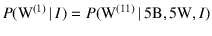
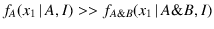
- ... probable,
- Please compare this expression,
“the extraction of White becomes more probable”, with
“the probability we assign to it”, used above. The former should
be, more correctly, “we assign higher probability
to the extraction of White”, as it will be clear later.
For sake of conciseness and avoiding pedantry, in this paper
I will often use imprecise expressions of this kind,
as used in every day language.
.
.
.
.
.
.
.
.
.
.
.
.
.
.
.
.
.
.
.
.
.
.
.
.
.
.
.
.
.
.
- ... waving.
- See
e.g. https://www.youtube.com/watch?v=YrsP-h2uVU4
from 48:00
(in Italian).
.
.
.
.
.
.
.
.
.
.
.
.
.
.
.
.
.
.
.
.
.
.
.
.
.
.
.
.
.
.
- ... out.
- Here is the result with a single line of R code:
> N=5; n=20; i=0:N; pii=i/N; pii^n/sum(pii^n)
[1] 0.000000e+00 1.036587e-14 1.086940e-08 3.614356e-05 1.139740e-02 9.885665e-01
(And, by the way, this is a good example of the importance
of a formal guidance in assessing probabilities: according to my experience,
after a sequence of 5-6 White,
people are misguided by intuition and tend to believe
box  much more than they rationally should.)
.
.
.
.
.
.
.
.
.
.
.
.
.
.
.
.
.
.
.
.
.
.
.
.
.
.
.
.
.
.
- ... get
-
Here is the R code for the example of 20 extractions resulting in 5 White:
> N=5; n=20; i=0:N; pii=i/N; x=5; pii^x * (1-pii)^(n-x) / sum( pii^x * (1-pii)^(n-x) )
[1] 0.000000e+00 6.968411e-01 2.979907e-01 5.167614e-03 6.645594e-07 0.000000e+00
(Note how using this code we can focus on the essence of what it is going
on, instead of being `distracted' by the math of the normalization.)
.
.
.
.
.
.
.
.
.
.
.
.
.
.
.
.
.
.
.
.
.
.
.
.
.
.
.
.
.
.
- ...Laplace:
- In the light of
Brecht's quote by Galileo you might be surprised to find quite
some quotes in this paper. But there are books and books.
.
.
.
.
.
.
.
.
.
.
.
.
.
.
.
.
.
.
.
.
.
.
.
.
.
.
.
.
.
.
- ...
likely,
- This would have been the correct answer to a different
question: probability of White from a box taken at random
among boxes
 ,
that is
,
that is  . Ruling out
  by hand at the very
beginning is quite different from ruling it out as a consequence
of the described experiment. The status of information is different
in the two cases and also the resulting probabilities will usually be
different! [Please note that a different state of information might
change probability, but not necessarily it does.
For example
by hand at the very
beginning is quite different from ruling it out as a consequence
of the described experiment. The status of information is different
in the two cases and also the resulting probabilities will usually be
different! [Please note that a different state of information might
change probability, but not necessarily it does.
For example
 just by symmetry.
Conditioning is subtle!]
just by symmetry.
Conditioning is subtle!]
.
.
.
.
.
.
.
.
.
.
.
.
.
.
.
.
.
.
.
.
.
.
.
.
.
.
.
.
.
.
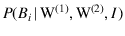
- ... get
- Here is the numerical result obtained with R:
> N=5; i=0:N; pii=i/N; ( PBi = pii/sum(pii) ); sum( pii * PBi )
[1] 0.00000000 0.06666667 0.13333333 0.20000000 0.26666667 0.33333333
[1] 0.7333333
.
.
.
.
.
.
.
.
.
.
.
.
.
.
.
.
.
.
.
.
.
.
.
.
.
.
.
.
.
.
- ... it.
- Curiously,
for strict frequentists
the probability that
 contains
  white balls
makes no sense because, they say, either it does or it doesn't.
white balls
makes no sense because, they say, either it does or it doesn't.
.
.
.
.
.
.
.
.
.
.
.
.
.
.
.
.
.
.
.
.
.
.
.
.
.
.
.
.
.
.
- ....
- The notation used above is consistent
with this statement, in the sense that the conditions
appearing in
 ,
,
 and
and
 can be seen seen as
  evolving with time.
.
.
.
.
.
.
.
.
.
.
.
.
.
.
.
.
.
.
.
.
.
.
.
.
.
.
.
.
.
.
- ... `objective'.
- It is curious to remark
that there
are, or at least there were,
also Bayesians `afraid' of subjective probability (7).
.
.
.
.
.
.
.
.
.
.
.
.
.
.
.
.
.
.
.
.
.
.
.
.
.
.
.
.
.
.
- ...,
- Note
also this very last statement, to which we shall return
at the end of the paper.
.
.
.
.
.
.
.
.
.
.
.
.
.
.
.
.
.
.
.
.
.
.
.
.
.
.
.
.
.
.
- ....
- As a real example, in my talk
at MaxEnt 2016 I analyzed the football match France-Portugal,
played right on the first day of the workshop, so that
everybody (interested in football) had fresh in their minds
the reaction of fans of the two teams, as shown on TV,
and also that of people in pubs in Ghent
(slides are available at
http://www.roma1.infn.it/~dagos/prob+stat.html#MaxEnt16_2).
.
.
.
.
.
.
.
.
.
.
.
.
.
.
.
.
.
.
.
.
.
.
.
.
.
.
.
.
.
.
- ... although
- What Hume says about
probability reminds me of the famous reflection by Augustine of Hippo
about time: “Quid est ergo tempus? Si nemo ex me quaerat, scio; si quaerenti explicare velim, nescio.“ - “What then is time? If no one asks me, I know what it is. If I wish to explain it to him who asks, I do not know.”
(https://en.wikiquote.org/wiki/Augustine_of_Hippo.)
Indeed, as a creature living in a
hypothetical Flatland
has no intuition of
how a 3D world would be, so a hypothetical intelligent humanoid
`determinoid,' living in a (very boring) world
in which all phenomena happen with extreme regularity, would
have not developed the concept of probability.
.
.
.
.
.
.
.
.
.
.
.
.
.
.
.
.
.
.
.
.
.
.
.
.
.
.
.
.
.
.
- ... black.
- The exact number of
 is 90.4%, as it can be easily checked
with R:
is 90.4%, as it can be easily checked
with R:
> N=5; n=4; i=0:N; pii=i/N; ( PBi=pii^n/sum(pii^n) ); sum(pii * PBi)
[1] 0.00000000 0.00102145 0.01634321 0.08273749 0.26149132 0.63840654
[1] 0.9039837
.
.
.
.
.
.
.
.
.
.
.
.
.
.
.
.
.
.
.
.
.
.
.
.
.
.
.
.
.
.
- ...
event.”
- The second
position, popularized by Einstein's “God does not play dice”,
is related to the so-called Laplace Demon,
“An intellect which at a certain moment would know all forces
that set nature in motion, and all positions of all items of
which nature is composed, if this intellect were also vast
enough to submit these data to analysis,
it would embrace in a single formula the movements
of the greatest bodies of the universe and those of the tiniest atom;
for such an intellect nothing would be uncertain and the future just
like the past would be present before its eyes.” (2)
.
.
.
.
.
.
.
.
.
.
.
.
.
.
.
.
.
.
.
.
.
.
.
.
.
.
.
.
.
.
- ... neutral).
- The branching ratios
of K
 into the two `channels' are
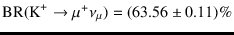 and
and
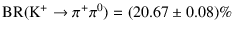 (12).
(12).
By the way, I do not think that Quantum Mechanics needs special rules
of probability. There the mysteries are related to the
weird properties of the wave function  . Once you apply the
rules - “shut up and calculate!” has been for long time
the pragmatic imperative -
and get `probabilities'
(in this case `propensities', as we shall see) all the rest
is the same as when you calculate `physical probabilities' in other systems.
Take for example the brain-teasing
single photon double slit experiment
(see e.g. https://www.youtube.com/watch?v=GzbKb59my3U).
From a purely probabilistic
point of view the situation is quite simple. Applying the rules of
Quantum Mechanics, if we open only slit
. Once you apply the
rules - “shut up and calculate!” has been for long time
the pragmatic imperative -
and get `probabilities'
(in this case `propensities', as we shall see) all the rest
is the same as when you calculate `physical probabilities' in other systems.
Take for example the brain-teasing
single photon double slit experiment
(see e.g. https://www.youtube.com/watch?v=GzbKb59my3U).
From a purely probabilistic
point of view the situation is quite simple. Applying the rules of
Quantum Mechanics, if we open only slit  we get
the pdf
we get
the pdf
 ; if we open only
  we get
 ; if we open both slits we get
 . Why should
be just a superposition of
and
? In fact within probability
theory there is no rule which relates them. We
need a model to evaluate each of them
and the best we have are the rules of Quantum Mechanics.
Once we have got the above pdf's all the rest follows
as with other common pdf's. In particular, if
we get e.g. that
. Why should
be just a superposition of
and
? In fact within probability
theory there is no rule which relates them. We
need a model to evaluate each of them
and the best we have are the rules of Quantum Mechanics.
Once we have got the above pdf's all the rest follows
as with other common pdf's. In particular, if
we get e.g. that
 we believe that
a photon will be detected `around'
we believe that
a photon will be detected `around'  , if we open only slit ,
much more than if we open both slits. And, similarly, if we plan to
repeat the experiment a large number of times,
we expect to detect `many more' photons `around' if
only slit is open than if both are.
That's all.
A different story is to get an intuition of the rules of Quantum Mechanics.
, if we open only slit ,
much more than if we open both slits. And, similarly, if we plan to
repeat the experiment a large number of times,
we expect to detect `many more' photons `around' if
only slit is open than if both are.
That's all.
A different story is to get an intuition of the rules of Quantum Mechanics.
.
.
.
.
.
.
.
.
.
.
.
.
.
.
.
.
.
.
.
.
.
.
.
.
.
.
.
.
.
.
- ...
particle.
- I like, as historian Peter Galison
puts it: “Experiments begin and end in a matrix of beliefs.
...Beliefs in instrument type, in programs of experiment
enquiry, in the trained, individual judgments about every local behavior
of pieces of apparatus.” (13) Then beliefs are propagated
within the scientific community and then outside.
But, as recognized, methods
from `standard statistics' (first at all the infamous p-values)
tend to confuse even experts and spread unfounded beliefs
through the scientific community as well as
among the general public (4,5), that in the meanwhile
is developing `antibodies'
and is beginning to mistrust striking scientific results and, I am afraid,
sooner or later also scientists and Science in general.
.
.
.
.
.
.
.
.
.
.
.
.
.
.
.
.
.
.
.
.
.
.
.
.
.
.
.
.
.
.
- ...preference)
- I have no strong preference on the name, and my
propensity in favor of `propensity' is because it is less used in
ordinary language (and despite the fact that this noun
is usually associated to Karl Popper,
an author I consider quite over-evaluated).
.
.
.
.
.
.
.
.
.
.
.
.
.
.
.
.
.
.
.
.
.
.
.
.
.
.
.
.
.
.
- ...physical
- Note the extended meaning of `physical',
not strictly related to Physics, but to `matters of fact' of all kinds,
including for example biological, sociological or economic systems
believed to have propensities to behave in different ways.
.
.
.
.
.
.
.
.
.
.
.
.
.
.
.
.
.
.
.
.
.
.
.
.
.
.
.
.
.
.
- ....
- I had heard
that this apparent obvious statement goes under the name
of Lewis' Principal Principle
(see e.g. http://plato.stanford.edu/entries/probability-interpret/).
Only at the late stage of writing this paper
I bothered to investigate a little
more about that `curious principle' and found out
Lewis' Subjectivist's Guide
to Objective Chance (14), in which his very basic concepts,
outlined in a couple of dozen of lines at the beginning
of the article, are amazingly in tune
with several of the positions I maintain here.
.
.
.
.
.
.
.
.
.
.
.
.
.
.
.
.
.
.
.
.
.
.
.
.
.
.
.
.
.
.
- ...:
- It becomes now clear the meaning
of Equation (7), which we can rewrite
as
having assumed a continuity of propensity values, and
having started our inference from a uniform prior, that is
 .
.
The normalized version of the above equation is
.
.
.
.
.
.
.
.
.
.
.
.
.
.
.
.
.
.
.
.
.
.
.
.
.
.
.
.
.
.
- ... presently),
- Here
is, for example, what David Lewis (see Footnote
23) writes in Ref. (14) (italics original):
“Carnap did well to distinguish two concepts of probability,
insisting that both were legitimate and useful
and that neither was at fault because it was not the other.
I do not think Carnap chose quite the right two concepts,
however. In place of his `degree of confirmation', I would put
credence or degree of belief; in place
of his `relative frequency in the long run', I would put chance
or propension, understood as making sense in the single case.”
More or less what I concluded when I tried to read Carnap
about twenty years ago: his first choice means nothing (or at least
it has little to do with probability); the second
does not hold, as I am arguing here.
.
.
.
.
.
.
.
.
.
.
.
.
.
.
.
.
.
.
.
.
.
.
.
.
.
.
.
.
.
.
- ... `trials'),
- To make it clear,
what is important to is that
 is (about) the same,
and that our assessments are independent. It does not matter
if, instead, the events have a different meaning, like e.g.
tails tossing a coin, odd number rolling a die, and so on.
The emphasized `about' is because itself could be
uncertain, as we shall see later. In this case we need to
evaluate the expectation of
is (about) the same,
and that our assessments are independent. It does not matter
if, instead, the events have a different meaning, like e.g.
tails tossing a coin, odd number rolling a die, and so on.
The emphasized `about' is because itself could be
uncertain, as we shall see later. In this case we need to
evaluate the expectation of  taking into account the
uncertainty about .
taking into account the
uncertainty about .
.
.
.
.
.
.
.
.
.
.
.
.
.
.
.
.
.
.
.
.
.
.
.
.
.
.
.
.
.
.
- ....
- Related to this there is the
usual confusion between a probability distribution and a distribution
of frequencies. Take for example
a quantity that can come in many possibilities, like
in a binomial distribution with
 and
and  .
We can think of repeating the trials a large number
of times and then, applying Bernoulli's theorem
to each of the eleven possibilities, we consider it very unlikely
to observe values of relative frequencies in each `bin'
different from the probabilities evaluated from the binomial
distribution. This is why we highly expect - and we
shall be highly surprised at the contrary! - a frequency distribution
(`histograms') very similar in shape to the
probability distribution, as you can easily `check' playing with
.
We can think of repeating the trials a large number
of times and then, applying Bernoulli's theorem
to each of the eleven possibilities, we consider it very unlikely
to observe values of relative frequencies in each `bin'
different from the probabilities evaluated from the binomial
distribution. This is why we highly expect - and we
shall be highly surprised at the contrary! - a frequency distribution
(`histograms') very similar in shape to the
probability distribution, as you can easily `check' playing with
n=10000; x=rbinom(n, 10, 0.5); barplot(table(x)/n, col='cyan')
barplot(dbinom(0:10,10,0.5), col=rgb(1,0,0,alpha=0.3), add=TRUE)
That's all! Nothing to do
with the “frequency interpretation of probability”,
or with the “empirical law of Chance”
(see Footnote 28).
.
.
.
.
.
.
.
.
.
.
.
.
.
.
.
.
.
.
.
.
.
.
.
.
.
.
.
.
.
.
- ....”
- Obviously, if you
make an experiment of this kind, tossing
regular coins or dice a large number of times,
you will easily find relative frequencies of a given face
around 1/2 or 1/6, respectively
as simulated with this
line of R:
p=1/2; n=10^5; sum( rbinom(n, 1, p) ) / n
But it is just because, in the Gaussian large number approximation,
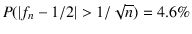 ,
and therefore
will
usually occur around
,
and therefore
will
usually occur around  [although all
  values
between 0 and 1 are possible,
with probabilities
values
between 0 and 1 are possible,
with probabilities
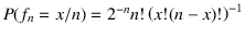 ].
Not because
there is a kind of `law of nature'
- “legge empirica del caso”, in Italian books,
i.e. “empirical law of Chance” - `commanding' that
frequency has to tend
to probability, thus supporting the popular
lore of late numbers at lotto hurrying up in order to obey it.
In the scientific literature and in text books, not to speak
about popularization books and article, it should be strictly
forbidden to call `laws' the results of asymptotic theorems,
because they can be easily misunderstood.
[For example we read (visited 11/11/2016) in
https://it.wikipedia.org/wiki/Legge_dei_grandi_numeri
that “the law of large numbers, also called empirical law of chance or Bernoulli's theorem [...] describes ...”
(total confusion! -
see also https://en.wikipedia.org/wiki/Law_of_large_numbers
and
https://en.wikipedia.org/wiki/Empirical_statistical_laws).]
].
Not because
there is a kind of `law of nature'
- “legge empirica del caso”, in Italian books,
i.e. “empirical law of Chance” - `commanding' that
frequency has to tend
to probability, thus supporting the popular
lore of late numbers at lotto hurrying up in order to obey it.
In the scientific literature and in text books, not to speak
about popularization books and article, it should be strictly
forbidden to call `laws' the results of asymptotic theorems,
because they can be easily misunderstood.
[For example we read (visited 11/11/2016) in
https://it.wikipedia.org/wiki/Legge_dei_grandi_numeri
that “the law of large numbers, also called empirical law of chance or Bernoulli's theorem [...] describes ...”
(total confusion! -
see also https://en.wikipedia.org/wiki/Law_of_large_numbers
and
https://en.wikipedia.org/wiki/Empirical_statistical_laws).]
Moreover, it should be avoided to teach that e.g. probability 1/3
means that something will occur to 1/3 of the elements of a
`reference class', i) first because a false sense of regularity
can be easily induced in simple minds, which will then complain
that the “the probabilities were wrong” if no event of that
kind occurred in 9 times; ii) second
because such `reference classes' might not exist,
and people should be trained in understanding degrees of belief
referred to individual events.
.
.
.
.
.
.
.
.
.
.
.
.
.
.
.
.
.
.
.
.
.
.
.
.
.
.
.
.
.
.
- ...analogous
 is the success in the first trial,
  the success in the second trial, and so on. Speaking
about “the realization of the same event” is quite incorrect,
because events
the success in the second trial, and so on. Speaking
about “the realization of the same event” is quite incorrect,
because events  are different. They can be at most
analogous. We indicate here, instead, by
are different. They can be at most
analogous. We indicate here, instead, by  the generic future
event of the kind of -
the generic future
event of the kind of - , i.e. for example
 .
.
.
.
.
.
.
.
.
.
.
.
.
.
.
.
.
.
.
.
.
.
.
.
.
.
.
.
.
.
.
.
- ... past.
- It is a matter of fact that,
because of evolution or whatever mechanism you might think about,
the human mind always looks for regularities.
This is how
Hume puts it (italics original):
“Where different effects have been found to
follow from causes, which are to appearance exactly similar, all these
various effects must occur to the mind in transferring the past to the
future, and enter into our consideration, when we determine the
probability of the event. Though we give the preference to that which
has been found most usual, and believe that this effect will exist, we
must not overlook the other effects, but must assign to each of them a
particular weight and authority, in proportion as we have found it to be
more or less frequent.” (9)
.
.
.
.
.
.
.
.
.
.
.
.
.
.
.
.
.
.
.
.
.
.
.
.
.
.
.
.
.
.
- ... `better'
-
To get an idea, repeat several times the following lines
of R code which simulate
n extractions with re-introduction
from box ri,
calculate the number of White,
infer the probability of the box compositions,
and finally evaluate the probability of a next White
and compare it with the relative frequency.
There is no miracle in the result, it is
just that the probabilistic formulae
are using all available information in the best possible way:
N=5; i=0:N; pii=i/N; ri=1; n=100; s=rbinom(n,1,pii[ri+1]); ( x=sum(s) )
( PBi = pii^x * (1-pii)^(n-x) / sum( pii^x * (1-pii)^(n-x) ) )
cat(sprintf("P(W|sequence) = %.10f; x/n = %.4f \n", sum( pii * PBi ), x/n))
.
.
.
.
.
.
.
.
.
.
.
.
.
.
.
.
.
.
.
.
.
.
.
.
.
.
.
.
.
.
- ...
time.
- I would like to make a related comment
on another myth concerning the scientific method, according to which
“replication is the cornerstone of Science”.
This implies that, if we take this principle literally, much of what
we nowadays consider
Science is in reality non-scientific
(can we repeat measurements concerning a particular supernova,
or two particular black holes merging with emission of
gravitational waves?).
And if you ask, they will tell you that this principle goes back
to none other than Galileo, who instead wrote(15)
that
“The knowledge of a single effect acquired
by its causes opens our mind to understand
and ensure us of other effects
without the need of doing experiments”
(“La cognizione d'un solo effetto acquistata per
le sue cause ci apre l'intelletto a 'ntendere ed assicurarci
d'altri effetti senza bisogno di ricorrere alle esperienze”).
Doing Science is not just collecting
(large amounts of) data, but properly framing
them in a causal model of Knowledge.
.
.
.
.
.
.
.
.
.
.
.
.
.
.
.
.
.
.
.
.
.
.
.
.
.
.
.
.
.
.
- ... experiment.
- What is nice in this practical
session, instead of abstract speculations, is that the people
participating in the discussion have developed their degrees of beliefs,
and therefore, when the box is taken away, they cannot say that
what they were thinking (and feeling!) is not valid anymore.
.
.
.
.
.
.
.
.
.
.
.
.
.
.
.
.
.
.
.
.
.
.
.
.
.
.
.
.
.
.
- ... uncertainty.
- See e.g. Feynman's quote
at the end of the paper.
.
.
.
.
.
.
.
.
.
.
.
.
.
.
.
.
.
.
.
.
.
.
.
.
.
.
.
.
.
.
- ...
innocent?
- If you worry about
these issues, then you might be interested in the
Innocence Project, http://www.innocenceproject.org/.
.
.
.
.
.
.
.
.
.
.
.
.
.
.
.
.
.
.
.
.
.
.
.
.
.
.
.
.
.
.
- ... box.
- Note that many statements
concerning scientific and historical `facts' are of this kind.
.
.
.
.
.
.
.
.
.
.
.
.
.
.
.
.
.
.
.
.
.
.
.
.
.
.
.
.
.
.
- ... circle.”
- See e.g.
https://developer.android.com/reference/android/location/Location.html#getAccuracy()
.
.
.
.
.
.
.
.
.
.
.
.
.
.
.
.
.
.
.
.
.
.
.
.
.
.
.
.
.
.
- ... bet.
- Here is how
Laplace reported his uncertainty on value
of the mass of Saturn got by Alexis Bouvart:
“His [Bouvard] calculations give him
the mass of Saturn as 3,512th part of that
of the sun. Applying my
probabilistic formulae
to these observations,
I find that the odds are 11,000 to 1 that the error in this
result is not a hundredth of its value.” (2)
That is
 Note how the expression “the odds are,” indicates
he was talking of a fair bet, viz. a coherent bet.
Moreover it is self evident that
such a bet cannot be, strictly speaking, settled, but it rather had
an hypothetical, normative meaning.
(And Laplace was also well aware of the non linearity between
quantity of money and its `moral' value, so that
a bet with such high odds could never be agreed in practice
and it was just a strong way to state a probability.)
Note how the expression “the odds are,” indicates
he was talking of a fair bet, viz. a coherent bet.
Moreover it is self evident that
such a bet cannot be, strictly speaking, settled, but it rather had
an hypothetical, normative meaning.
(And Laplace was also well aware of the non linearity between
quantity of money and its `moral' value, so that
a bet with such high odds could never be agreed in practice
and it was just a strong way to state a probability.)
.
.
.
.
.
.
.
.
.
.
.
.
.
.
.
.
.
.
.
.
.
.
.
.
.
.
.
.
.
.
- ... fact,
-
“If we were not ignorant there would be no probability,
there could only be certainty. But our ignorance cannot
be absolute, for then there would be no longer any probability
at all. Thus the problems of probability may be classed
according to the greater or less depth of our ignorance.”
(18)
.
.
.
.
.
.
.
.
.
.
.
.
.
.
.
.
.
.
.
.
.
.
.
.
.
.
.
.
.
.
- ...
probabilities,
- Italians might be pleased to remember
Dante's “Cred'io ch'ei credette ch'io credesse che ...” (Inf. XIII, 25),
expressing beliefs of beliefs of beliefs
(“I believe he believed that I believed that...”),
roughly rendered in verses as “He, as it seem'd, believ'd,
that I had thought [that]...”
(https://www.gutenberg.org/files/8789/8789-h/8789-h.htm#link13).
.
.
.
.
.
.
.
.
.
.
.
.
.
.
.
.
.
.
.
.
.
.
.
.
.
.
.
.
.
.
- ... questions
- For example we can ask the range
of virtual coherent bets one could accept
in either direction, or `calibrate' probabilistic judgements
against boxes with balls of different colors (or other mechanical
or graphical tools).
.
.
.
.
.
.
.
.
.
.
.
.
.
.
.
.
.
.
.
.
.
.
.
.
.
.
.
.
.
.