Signal and background: a Mathematica example

As a last application of the Poissonian model, let us make a numerical example of a counting measurement in the presence of background. To compare full and approximative results, let us choose a number large enough for the normal approximation to be reasonable. For example, we have observed 44 counts with an expected background of 28 counts. What can we tell about the signal? We solve the problem with the following Mathematica code^9.3 applied to the formulae of Section ($s$ stands for $\lambda_s$ and $b$ for $\lambda_{B_\circ}$):

(********************************************************)
ClearAll["Global`*"]

f = (Exp[-s]*(b0+s)^x)/(x!Sum[b0^i/i!, {i, 0, x}])
 
x=44;
b0=28;

m = NIntegrate[s*f, {s, 0, 1E^6}]
sigma = Sqrt[NIntegrate[s^2*f, {s, 0, 1E^6}] - m^2]         
  
Plot[f, {s, 0, 50}, AxesLabel->{s, "f"}]

fd1=D[Log[f], s];
fd2= D[fd1, s];

res=FindMinimum[-f, {s,m}];
smax = res[[2]]
sigma2=1/Sqrt[-(fd2 /. res[[2]])]
(********************************************************)

The code evaluates and plots the final distribution of $\lambda_s$ obtained from a uniform prior [formula ()] and calculates:

• the prevision E$(\lambda_S)$
  m$$\equiv$$   E$$(\lambda_S) = 17.0\,;$$

• the standard deviation $\sigma(\lambda_S)$:
  sigma$$\equiv \sigma(\lambda_S) = 6.7\,;$$

• the mode $\lambda_{S_m}$:
  smax$$\equiv \lambda_{S_m} = 16.0 \,;$$

• the approximated standard deviation calculated from the shape of the final distribution around the mode (see Section ):
  sigma2$$= 6.6\,.$$

The resulting probability density function for the signal is shown in Fig. .

The approximate, but still Bayesian, reasoning to get the same result is as follows.

1. Given this status of information, the certain quantities are:
   • The average value of the background: $\lambda_{B_\circ}=28 \pm\approx 0$;
   • The observation $x=44$ (it does not even make sense to write $\pm 0$: 44 is 44 !).
2. Instead, we are uncertain on the parameter $\lambda$ of the Poissonian distribution responsible for the observed number of counts; we can infer [see () and ()]
   $$\lambda \approx x \pm \sqrt{x} = 44.0\pm 6.6\,.$$

3. Since $\lambda$ is due to the contribution of the signal and background, we have, finally:
   $$\lambda_S = \lambda - \lambda_{B_\circ} = 16.0\pm 6.6\,.$$

The last evaluation is an example of how Bayesian reasoning helps, independently of explicit use of Bayes' theorem. Nevertheless, these results are still conditioned by the assumption that the signal looked for exists. In fact, Fig. does not really prove, from a logical point of view, that the signal does exist, although the distribution seems so nicely separated from zero (see also Ref. [25]).

Figure: Final distribution for the signal ( 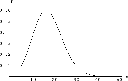$s\equiv \lambda_S$), having observed 44 counts, with an expected background of 28 counts.