Probabilistic Inference and Forecasting in the Sciences
lectures to PhD students in Physics (39o Ciclo)
(Giulio D'Agostini and
Andrea Messina)
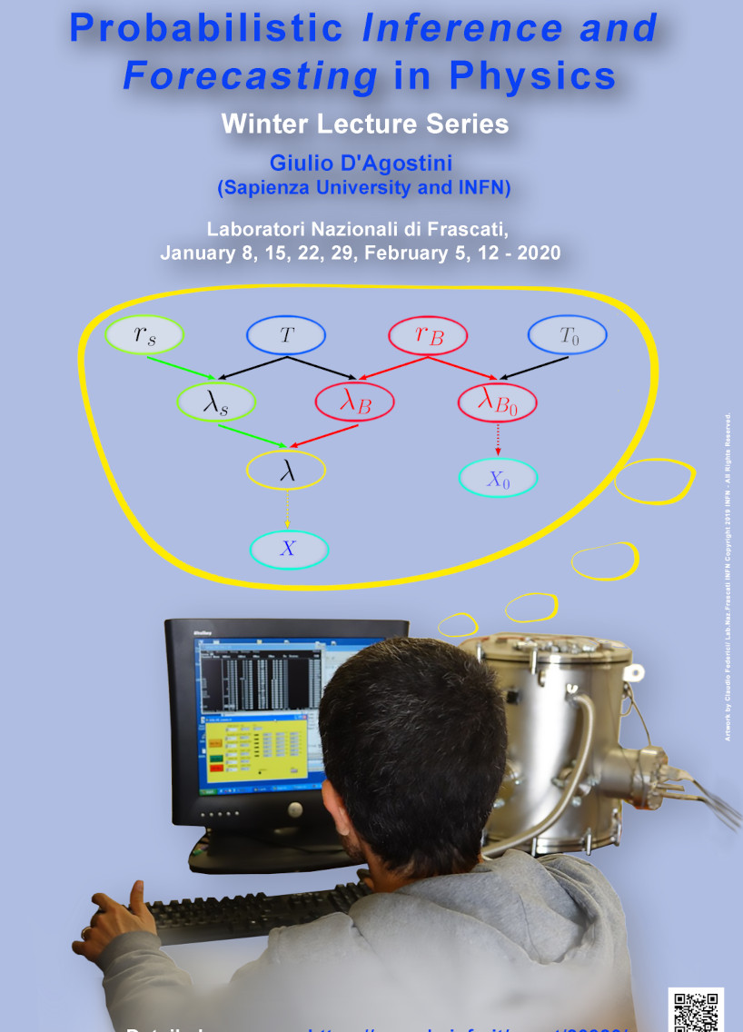
[Poster for lectures at LNF]
The course will be of about 40 hours (6 credits),
Contents
Time table
(*) Seminar on 30 years of Bayesian unfolding
- Lecture 1 (8 January)
- Introduction to the course and entry test
in particular (although at qualitative level)
- models, model parameters ('μ', 'λ', 'p', etc.)
and empirically observed quantities ('x');
- measurement as a probabilistic inferential problem:
- ranking in probability the possible numerical values of the model parameters.
- Probabilistic inference and probabilistic forecasting
- A paradigm shift in data analysis from the old `formulae oriente approach'.
- Discussion (mainly qualitative) on some of the problems: nr. 1, 7 and 15.
References, links, etc.
- Lecture 2 (10 January)
-
- Continuing with the entry test:
→ discussion (mainly qualitative) on some of the problems: nr. 6, 11 and 13.
- What we di when we do measurements
- from 'observed' values on instruments
... to the values of physical quantities;
- measurement models.
- Sources of uncertainty
- ISO/GUM dictionary,
— in particular, error ≠ uncertainty (!!)
— some details on source nr. 5, with some 'related' topics
of hystoric interest
— (see links and references below
— Physics facts and ideas are often interconnected!)
- Type A and
Type B uncertainties
- 'Usual' (old style) handling of uncertanties.
- A simple case (related to nr. 3 of the entry test):
inferring a physical quantity
associated with the parameter μ of a Gaussian
error distribution,
having observed a large sample sample
and assuming that
- μ does not change during the measurements;
- there are not 'systematic errors' (the only source
of uncertanty is nr. 10 of the GUM list).
References, links, etc.
- ISO GUM
(see also
here)
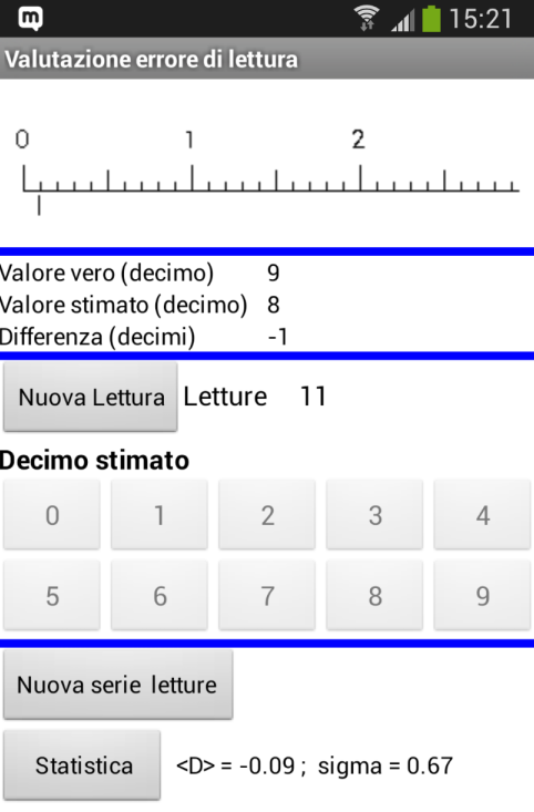
- Android app to check your ability
to interpolate between scale marks
- ErroriLettura.apk
(screenshot)
- No dogmatism, please!
- Remark: skill to interpolate between scale marks
was foundamental for a correct use of a
slide rule
- Other apps from Google app store:
- Extra links and recomended readings somehow related to the subject:
A cultural/scientific must, mentioned during the lecture
Lecture 3 (12 January)
- Probabilistic statements of the numerical value physical quantities
vs confidence intervals
and coverage
(somehow qualitative, as in invitation to think about and, as far
the 'frequentistic' terms are concerned,
to look in the preferred
books and lecture notes).
- Causes → Effects, and back.
- Simple example with two Causes and two effects (AIDS test).
- P(A|B) vs P(B|A).
- 'Prosecutor fallacy' (aka base rate fallacy,
base rate neglect and base rate bias).
- What is 'statistics'? [→"Lies , dammn lies and statistics"]:
descriptive statistics, probability theory, inference.
- "Lies, damned lies and... Physics":
claimes of discoveries based on 'p-values' ('n-σ')
References, links, etc.
- GdA, About the proof of the so called exact classical confidence intervals. Where is the trick?,
arXiv:physics/0605140 [physics.data-an]
- Is Most Published Research Wrong?,
YouTube
by Veritasium (very well done!),
based on
- J. Bohannon, I Fooled Millions Into Thinking Chocolate Helps Weight Loss.
Here's How,
GIZMODO 27 May 2015
Some related material:
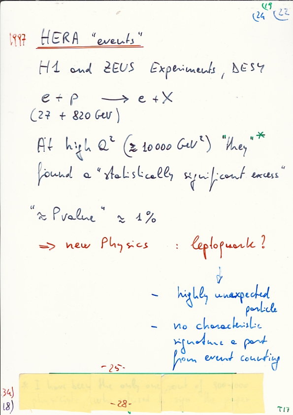
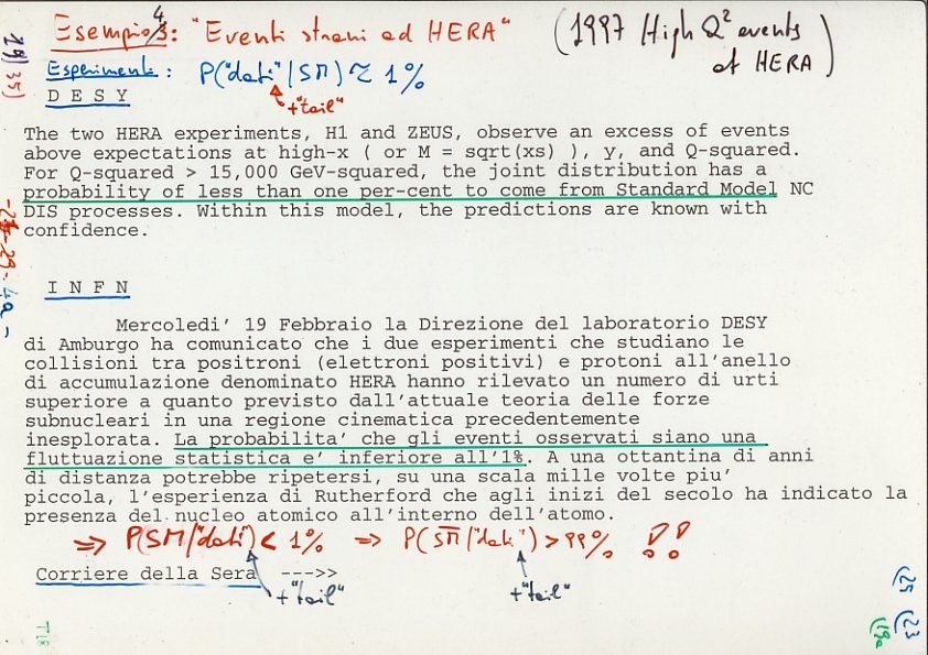
- For (just) an example, from Medical Science, on results reported
quoting p-values:(*)

- An `important' case
(1997, appearing in GdA curriculum as antipublication)
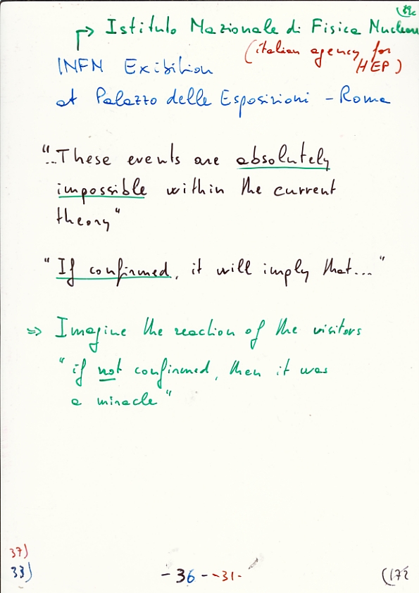
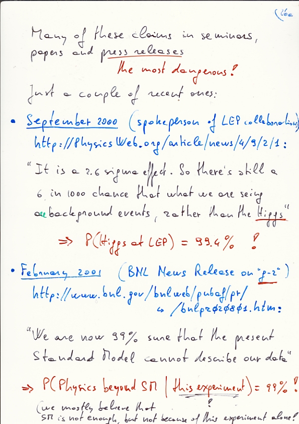
- Other old (2000,2001) claim of discoveries based on 'sigmas',
one of which even concerned the Higgs particle (old style slides):
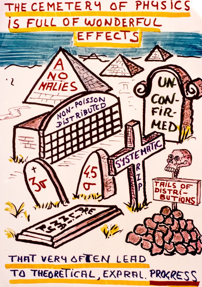
(Much later the 1984 de Rujula's Cemetery of Physics,
and many more claims have followed...)
Lecture 4 (15 January)
- Entry test: nr. 10, with qualitative discussion on related concepts:
- inferring several physical quantities from the same dataset;
- they are, in most cases `correlated', i.e. 'not independent';
- reconditioning the value of some quantities on the 'assumed
exact value' of the others
(but also uncertainty on the
conditionand can be taken into accout).
- Special case of two quantities, e.g. m and p
resulting from a linear fit:
- graphical representation of the result in the
(m,p) plane;
- graphical meaning of the correlation;
- reason why if the data points (x and y)
are in the first quadrant then ρ is negative
(→ m and p anticorrelated)
Blackboard
- Probability of hytheses vs 'classical' hypothesis tests
- More on χ2: see last slide of previous lecture (updated)
- Mechanism behind the 'classiical' hypothesis tests:
- from falsificationism to p-values
... and misundestandings(!!)
- Doing logical mistakes and crimes with p-values:
- Examples of p-values based on χ2
References, links, etc.
Lecture 5 (17 January)
- Learning from data: model thinking
- A toy experiment: six boxes, each containing five balls:
- Probability of the box composition;
- Probability of the next extraction
(we have analysed, for the moment, the case of 'reintroduction')
It will be the guide examples for many concepts of the course
- Ellsberg paradox (shown without mentioning the name)
- What/where is probability?
- Subjective nature of probability:
- Probability is always conditioned probability
- P(E|Is(t))
- Role of bets, and in particular of coherent bets,
in order to express the 'degree of belief' ('of certainty', etc.)
- On the standard (old) textbook 'definitions' of probability
- Basic rules of probability (3+1):
for the moment, just a reminder, with clarifications
- Rule to update the probability in the light
of a new piece of information:
→ just a mathematical manipulation of the forth basic rule
→(no membership to a sect required...)
→ Bayes' theorem, or 'rule'
→(indeed, calling it 'theorem' is perhaps too much;
calling it 'principle' shows mental confusion...)
Lecture 6 (19 January)
- From the basic rules of probabilities
to the Laplace's "Bayes Theorem"
- Proposed problems:
- Aids test
- Three boxes and two rings
- Particle identification
- Six box toy experiment:
- analysis of the experimental data (5 times Black):
→evolution of the probabilities of the box composition;
→ evolution of the probability of the next Black
(BUT remember that the box composition remains constant:
WHERE IS PROBABILITY?)
- Homework at pag. 14 of the slides
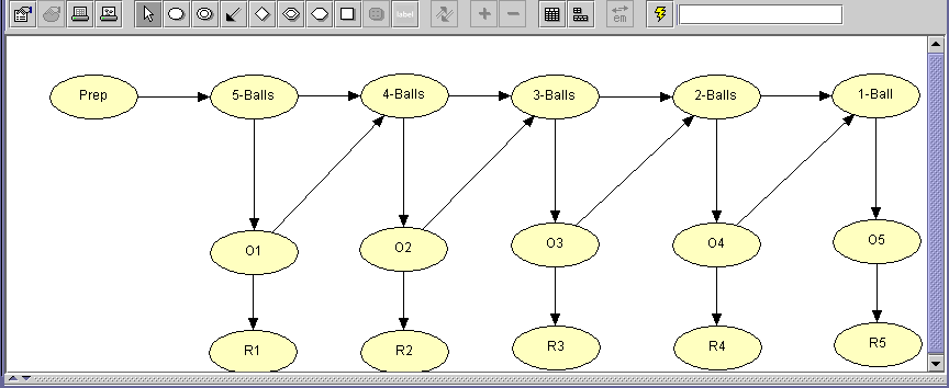
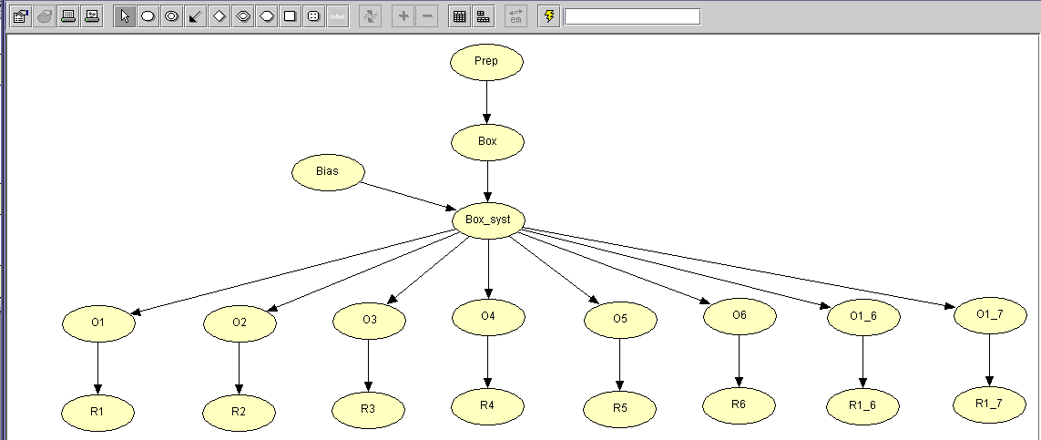
- Playing with Hugin
(six box problem, with variations, framed in a
Bayesian network)
- On the intuitive evaluations of probability
(following David Hume, with caveats concerning
induction)
- "Bayes' factor" (conceptual tool proposed by Gauss!)
References, links, etc.
- Veritasium on Bayes theorem
- GdA, The Gauss' Bayes Factor,
arXiv:2003.10878 [math.HO]
(See also here for historical related issues)
- Th. Cathcart and D. Klein,
Plato and a Platypus Walk into a Bar
(recensione su Scienza Per Tutti)
- GdA, Teaching statistics in the physics curriculum.
Unifying and clarifying role of subjective probability,
AJP 67, issue 12 (1999) 1260-1268;
arXiv:physics/9908014
(local pdf file)
[limited
to Sections II and IV, for the moment]
- Hugin:
Hugin Lite (free → download)
- Tutorials.
- Examples provided by the company:
Samples
- Ready-to-use models based on the six-boxes toy experiment:
- Try to edit the models
(within HUGIN), changing the probability
tables, adding nodes, etc..
- Try to write from scratch the (minimalist) model to solve
the AIDS problem, using the number suggested in the slides
for easy comparison.
just two nodes
- Infected, with two possible states,
Yes and No;
- Analysis result, with two possible states,
Positive/ and Negative.
- Modify the previous model, using equiprobable
priors for Infected/Non-Infected:
- compare the result with the those obtained
with (roughly) realistic priors;
- compare the result with the wrong one suggested
in the first lecture.
- Think then to the possible practical utility of
using equiprobable priors.
- Netica: a valid alternative to Hugin,
thanks also to the many available
whose interest goes beyond the specific package.
- S. Cenatiempo, GdA e A. Vannelli,
Reti Bayesiane: da modelli
di conoscenza a strumenti inferenziali e decisionali
Lecture 7 (22 January)
- Six boxes analysied by HUGIN:
suggested variations (no code provided — try it)
- Uncertain numbers — an introduction.
- More about the importance of the state of information
in our scientific judgements (cows and sheep jokes).
- Extending the past to the future
(possibly avoiding the end of the inductivist turkey...).
- Uncertain numbers and probability distributions
- Summaries of probability distribution
(do not confuse RMS with σ!)
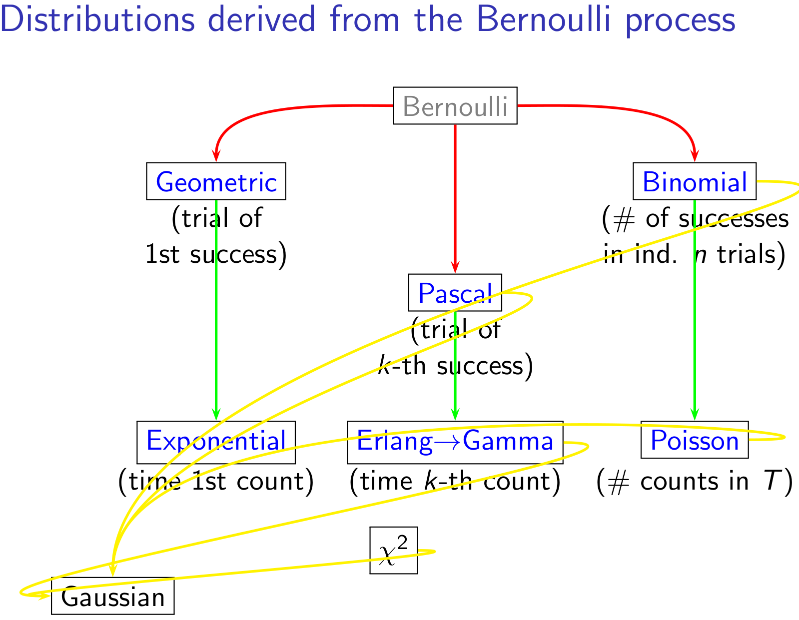
- Bernoulli process and related distributions
(Geometric, Binomial and Pascal).
- Introduction to Monte Carlo sampling using basic techniques:
- hit/miss
- inverting the cumulative distribution
(techniques introduced on discrete distribution
and easily/better extended to continuous distributions)
Write (pseudo-)random number generators for
- f(x) ∝ x (0 ≤ X ≤ 1)
- f(t) ∝ e-t/τ (0 ≤ T < ∞)
- f(x) ∝ cos(x) (-π/2 ≤ X ≤ π/2)
- X ∼ B10,1/5 (binomial distribution with n=10 and p=1/5)
[Note: in the cases 1, 3 and 4 use both techniques we have seen;
in the case 2 we can only use the "F-1(yR)" technique]
- From the Bernoulli process to the Bernoulli theorem:
- Bernoulli distribution
- Geometric distribution
- Pascal distribution (no details for the moment)
- Binomial distribution
- Bernoulli theorem: "p → fn"
References, links, etc.
Lecture 8 (24 January)
- Poisson process and related distributions
(Poisson, Exponential and Erlang).
→ Entry test nr. 8
- Bernoulli theorem: meaning and misundestrandings.
- decay lifetime vs half time of
radioactive decays.
- Markov and Cebicev disequalities
- Continuous probability distributions
with some important ones
- (negative) exponential;
- uniform;
- triangular (symmetric and asymmetric)
- Gaussian
References, links, etc.
Lecture 9 (26 January)
- The 'Gaussian trick' (Laplace approximation — !! )
- Propation of uncertainties: general problem and minimal solution
- Central Limit Theorem and its importance (it plays a central role)
- Reproductivity property of some distributions
- Exact, approximate and MC propagation of uncertainties
- Criticism concerning `propagation prescriptions'
- Introduction to multivariate distributions ('uncertain vectrors')
- Chain rule and its importance
- Probabilistic dependence/independence and covariance
References, links, etc.
- ...
- GdA, Bertrand 'paradox' reloaded,
https://arxiv.org/abs/1504.01361
→ besides the 'paradox', the paper
contains details on exact tranformations of variables.
- GdA, Asymmetric Uncertainties: Sources, Treatment and Potential Dangers,
https://arxiv.org/abs/physics/0403086
- PDF of sum of two ('iid') asymmetric triangular distributions
done analytically using Mathematica:
[But it can be done more easily by MC, also extending it to many
triangulars, using rtriang()
included in the script triang.R
available in the R web page]
Lecture 10 (29 January)
- Logical vs probabilistic(*) dependence/independence
(examples in the slides just sketched: → work out the details)
(*) Note: in the slides the adjective 'stochastic' is often
used, but I tend now to prefer the Latin root.
- About the transitivity of probabilistic(*)
dependence/independence
(examples in the slides just sketched: → work out the details)
- Some remarks on updating probabilities:
↠ P(B) is modified, in percentage, by hypothesis A
↠ as P(A) is modified, in percentage, by hypothesis B.
- More on exact propagations:
- work out the assigned problems (before reading the solutions on the slides);
- alternative method (wrt to that using the Dirac delta) for
variables monotonically related;
- mathematical transformation functions equal to the cumulative:
- the resulting variables is uniformelly distributed;
- exercise: prove it ising the 'Dirac delta' method.
- Waiting time for 'k' counts in a Poisson process:
- Erlang distribution;
- from Erlang distribution to Gamma distribution;
- Summary of distributions arising from the Bernoulli process
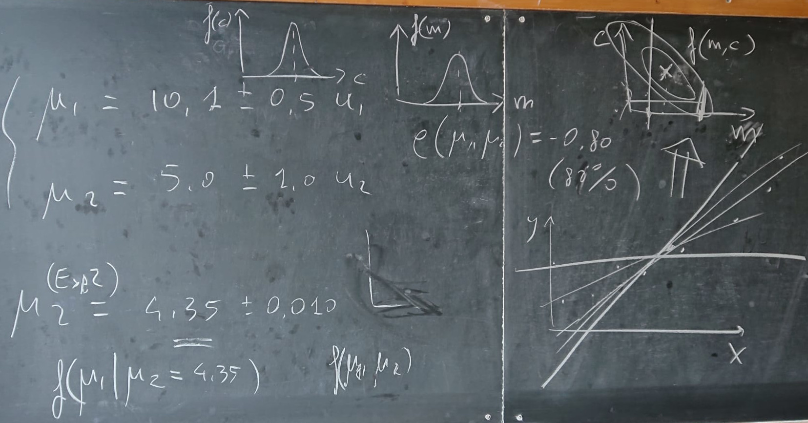
- Some related problems on Gaussian distributions
- Bivariate normal distribuion
→ Problem nr 10 of the entry test
References, links, etc.
- Today's slides
- GdA, usual lecture notes in Italian
- GdA, Learning about probabilistic inference and
forecasting by playing with multivariate normal distributions
(with examples in R),
https://arxiv.org/abs/1504.02065,
Secs. 1-2.6.
In particular → proof of the expression of the conditional distribution,
Sec 2.5.1
(left to self study)
Lecture 11 (31 January)
- Complementing the exponential, based on the following exercise:
- given a pdf f(x) ∝ K*exp[-α x^2 + β x],
with K and α positive, find
without making integrals
(and tell which kind of distribution we are dealing with).
- 'Gaussian Trick' in 2 dimensions (use and misuse)
- Extension of the bivariate normal to n dimensions:
multidimentional reconditioning.
- More on linear combinations of uncertain numbers
↠ 'Propagation' of covariance matrix
- Propagation via linearization;
- Special case of monomial functions
References, links, etc.
- Today's slides
- GdA, usual lecture notes in Italian
- GdA, Learning about probabilistic inference and
forecasting by playing with multivariate normal distributions
(with examples in R),
https://arxiv.org/abs/1504.02065,(*)
- up to Sec. 3,
with invitation reproduce the function norm.mult.cond() in your preferred language.
- Sec. 9.1 on how to constrain the sum of internal angles of a triangle
— problem mentioned during the lecture.
- Multivariate normal distribution (Wiki)
→ Conditional distributions
- Problems suggested in the slides:
rm23_07_problems.pdf
(The meaning of the last exercise will be clear next time.
For the moment just take a a generic pdf in the variable p.)
(*)
Note: Ref. 3 (M. Eaton, Multivariate Statistics...)
is no longer available in the website indicated there.
However
- the formulae for multivariate conditioning (see slides) can be found on Wiki (see above);
- the book can be found on an
alternative
link (visited 31 Janyary 2024; but pdf download not available)
and, moreover, the book is VERY formal — NOT recommended.
Lecture 12 (2 February)
- A first look at JAGS/rjags for MC simulation
→ try to translate the examples in Python and/or Julia
- Back again to the six boxes
→ simulations and comparison with frequency based
evaluations of probabilities
- Inferring p of Bernoulli processes
- Inferring p of a binomial distribution and inference of the
number of successes in future trials
(assuming p constant although unknown — and if p
depends on time? Think about it!)
- Probability vs frequency:
- Bernoulli theorem: p → fn
- Laplace's rule of succession (via "Bayes Theorem"):
fn → p
- Conjugate prior → Beta distribution
- Predicting the number of successes in future trials.
- Special case in which no successes were observed
(but the experiment was performed)
→ Exercice proposed at p. 28 of the slides (very important
→ we shall come back to the issue)
- Inference and prediction related to Poisson processes
- Inferring Poisson λ (and 'r')
- Conjugate prior → Gamma distribution
- Predicting the number of counts in future measurements
(assuming constant 'r')
- Special case in which no events have been observed
(but the experiment was done!)
Solve the exercise similar to that proposed at p. 28 for the slides
[in this case the quantity of interest is
r = λ/T
→ plot f(r | x=0, f0=k) in log-log scale].
- Use of JAGS for inference and prediction (see examples below).
References, links, etc.
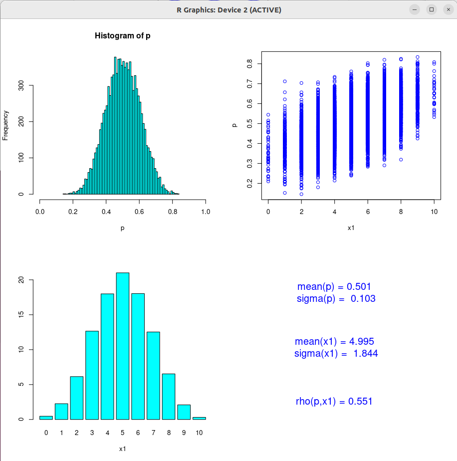
- JAGS/rjags(*) examples (see also dedicated web page)
- JAGS 'improperly' used as simple random generator:
In alternative, the model file can be defined inside the R script:
— simple_simulations_1.R
Moreovere, here is how to extract the individual histories and to make
customized graphics:
simple_simulations_graphics.R
(run the script after the previous one, and cuctomize it at wish).
[During the lecture we have also seen how to add variables x5 and x6,
related to x1 and x2]
- Other simple simulations:
- Inferential/predictive use, applied to Poisson processes
- Inferential/predictive use, applied to Bernoulli processes
→ Try, e.g., to change n0 and x0, keeping x0/n0 constant.
(*) For the moment take it as a kind of black box.
We shall see in the following lectures how it works.
And, 'obviously', there is also the equivalent of 'rjags' for Python:
PyJAGS
(it seems there also
'something' for Julia)
↠ Working Python and Julia
versions of the above examples are welcome!
- GdA, More lessons from the six box toy experiment,
arXiv:1701.01143 [math.HO]
→ see in particular footnote nr. 11 about Laplace's probability
of sun rising tomorrow
- GdA, Ratio of counts vs ratio of rates in Poisson processes,
arXiv:2012.04455 [stat.ME],
only Sec. 3.
Lecture 13 (12 February)
- Gaussian model assuming σ known:
- joint pdf of model parameters and observed values;
- inference of μ;
- predicting a future x;
- case of several 'independent' observations, with some remarks:
- observation on independency vs conditional independency;
- empirical observations vs measurements
(slide nr 17, to be commented in a following lecture);
- remarks on propagation of evidence
(case of 'divergent connections')
[for 'converging' and 'serial' connections see
arXiv:1504.02065 (Sec. 11)];
- conjugate prior.
- Joint inference of μ and σ (general considerations —
details left to self study)
- summary of 'large n behaviour;
- problem solved by JAGS
- Details on the rejection sampling ('hit/miss') for Monte Carlo.
- Importance sampling.
- Introduction to Markov Chain Monte Carlo
by playing with a three state toy model.
References, links, etc.
- Inference and prediction from a Gaussian sample (using JAGS/rjags):
- inf_mu_sigma_pred.R
— Which kind of prior does "dgamma(1.0, 1.0E-6)"
approximately model
— Modify the prior of of
τ=1/σ2 (*)
- still making use of a Gamma pdf;
- a) assuming an initial value of σ ≈ 10 ± 10 (mean and standard deviation);
- b) assuming an initial value of σ ≈ 1 ± 1 (mean and standard deviation).
(*) For a better comparison of the results
it is recommended to split code in the
several scripts:
- one to simulate the data
- others to analyze the same data using
different models/priors.
- More on priors:
- For an introduction to MCMC, Metropolis and Gibbs sampler:
C. Andrieu et al., An introduction to MCMC for Machine Learning,
Machine Learning, 50 (2003) 5-43,
https://doi.org/10.1023/A:1020281327116 (local copy)
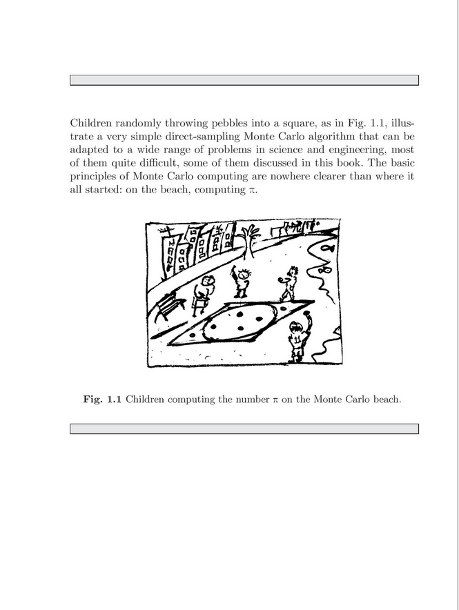
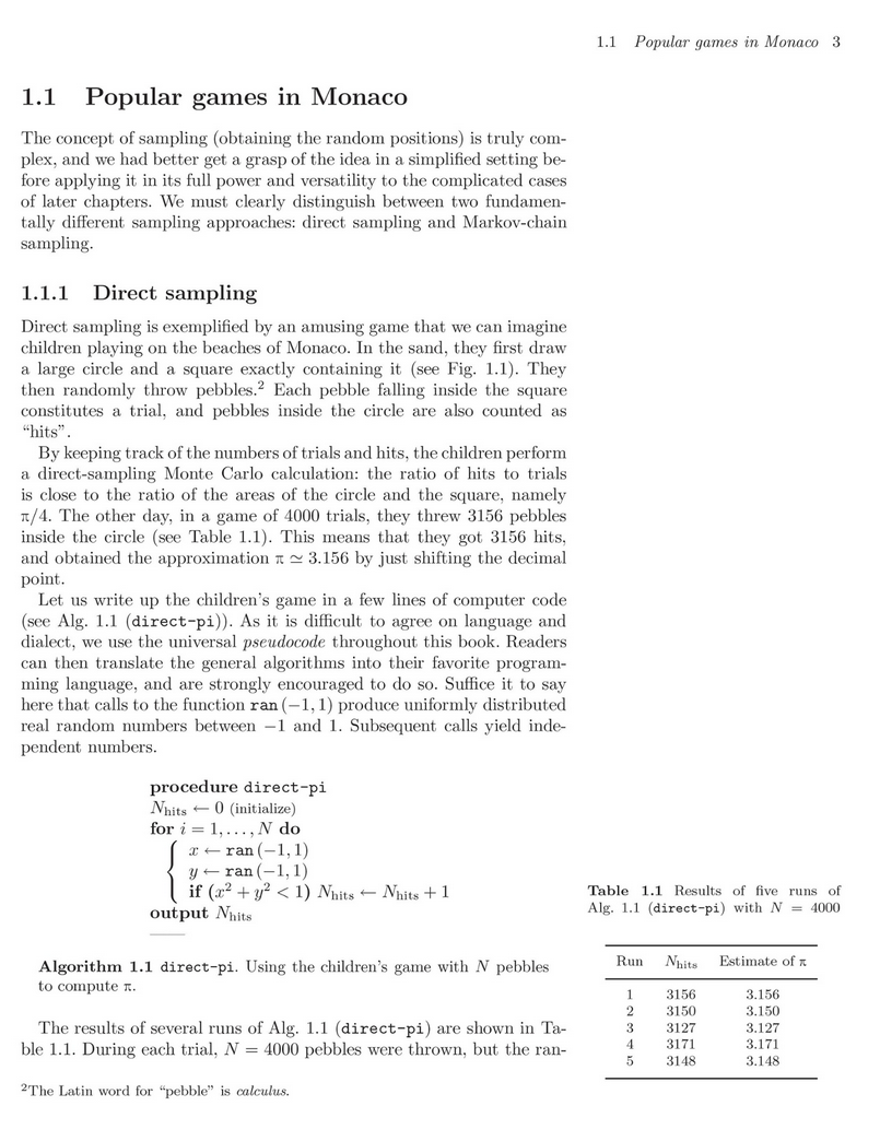
- The examples of children and adults playing throwing stones are from
Statistical
Mechanics: Algorithms and Computations by
Werner Krauth,(*)
with the relevant pages readable in the Amazon preview
- backup screenshots:
1,
2,
3,
4,
5,
6,
7,
8,
9
(*)An online course on the subject, with Krauth
as main instructor, available
on Coursera
- For Metropolis, Fermi & Co., see e.g.
in this hystoric excursus
and references therein.
- Lecture notes Probabilità e incertezze di misura,
Parte 4, Sec. 11.6
- R scripts concerning other MC issues, expecially MCMC:
Lecture 14 (14 February)
- Practical introduction to MCMC (focusing on data analysis):
- global and detailed balance conditions;
- Metropolis algorithm (with mention to Metropolis-Hasting);
- simulated annealing;
- Gibbs sampler.
- Simples examples of inference/forecasting making use of self-made MCMC's.
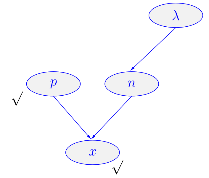
- Inferring n of a binomial given x and p.
- Framing the previous 'exercise' in a
more general model.
- Including in 'systematics' in the probabilistic model
- reminding ISO's influence quantities (h hereafter: → h);
- possible strategies:
- global inference on f(μ, h) followed by marginalization;
- conditional inference;
- inference of 'μR', followed
by propagation
(method particulary suited to get approximated formulae).
- Details on the systematics due to an uncertain offset in a Gaussian model:
- case of a single μ;
- influence of systematics in the result vs calibration
(μ known → z);
- case of several μ's measured with the same instrument
(same 'f(z)'), with details on two μ's
- f(μ1,μ2 | x1,x2),
in particular ρ(μ1,μ2).
References, links, etc.
- GdA, Bayesian reasoning in high-energy physics : principles and applications,
Secs. 5.6 and 2.10.3
(Report available at the CERN Document Server)
- GdA, Bayesian inference in processing experimental data:
principles and basic applications, Secs. 6 and 9
(Preprint: arXiv:physics/0304102)
- Concerning the BUGS project, to which JAGS is somehow related
- see here
- Interesting developments:
- For an introduction to MCMC and BUGS
- R scripts (some using JAGS)
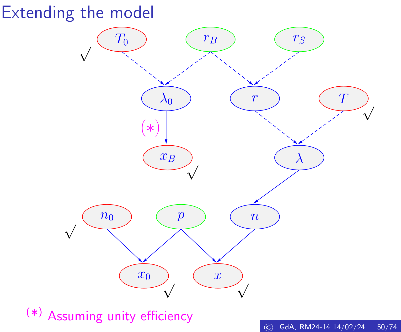
- Suggested variation of the script left as exercise (slides, p. 55):
- Extend the model in order to include
also the inference
of λ from which n derives (p. 44)
[Note: since n depends on the uncertain node λ,
the lower limit provided by ' I(nmin,)' is not needed
and not accepted by JAGS!]
- BAT
Lecture 15 (16 February)
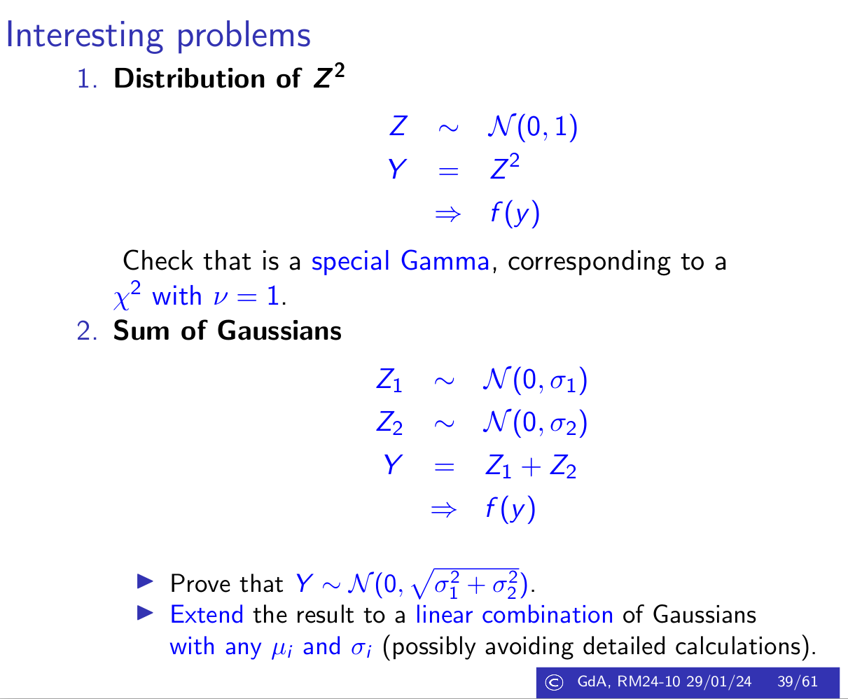
- Proposed exercises on exact approximations:
- sum of two Gaussians
- distribution of Z2, with Z ∝ N(0,1)
- Some problems involving binomial distributions related to Covid.
- Ratios of counts vs ratios λ's in Poisson processes.
- Uncertainties due to systematics
- Reminder of 'approach nr. 3';
- Application to offset and scale
systematics.(*)
- Fits (just parametric inference!):
- the importance of the underlying model;
- linear model: general approach; simplified
model (under well understood conditions) and
'least square' approximation
(no 'principles'!)
- case of uncertain σ;
- forecasting a future 'y' at a given xf.
(*) Note added :
as we have seen, the 'systematics' are related to influence quantities (ISO GUM).
Not only we can evaluate the contribution to the overall uncertainty due to the uncertain
value of the influence factors,
but, if there are good reasons to expect that a quantity can better measured in the future
(think to frontier Physics),
we can also provide, among the results, also the derivative of the
final value of interest wrt the the value of the uncertain input quantities.
As and example see
paper with Degrassi on the Higgs mass:
→ Tabs. 1-4.
References, links, etc.
- GdA, Checking individuals and sampling populations with imperfect tests,
arXiv:2009.04843
- GdA, What is the probability that a vaccinated person is shielded from Covid-19?,
arXiv:2102.11022
- GdA, Ratio of counts vs ratio of rates in Poisson processes,
arXiv:2012.04455
- GdA, CERN Yellow Report 99-03
- GdA, Fits, and especially linear fits ...,
arXiv:physics/0511182 ,
Secs. 1-2.
- GdA, Fit, in Italian,
(pdf version: Capitolo 12)
- GdA, Learning ... by playing with multivariate normal distributions
arXiv:1504.02065,
Sec. 10
- R scripts:
Suggested work:
- modify the script in order to:
- evaluate and plot also μy(xf)
-
modify further the script in order to:
- consider two extrapolations, one at xf1=30
and the other at xf2=32:
→ make the two plots, evaluate expected values and variances;
→ draw the scatter plot and evaluate the correlation
coefficient of yf(xf2) vs yf(xf1).
Lecture 16 (26 February) + Seminar on unfolding
- Two curious problems:
- two envelops: hold or change?
- three prisoner problem.
- Coherent bet and basic rules of probability.
- p-values vs Bayes Factors (and much more!)
(based on the real case of 2015 GW's)
- Back to basic probabilistic issues
- Probability and odds
- Coherent bets (de Finetti)
- Basic probability rules derived from coherence
- Expected gain in coherent bets
- Events and sets (and rules of probabilities)
- More on independence
- Relative update of probability
- Back to p-values:
- What they are
- What they are not
- p-values say very little (if not nothing) on the
probability of hypotheses
- 'Discovery' of Higgs particle (2011-2012) and
first detection on Earth of GW's
- More on Bayes factors and how they are (not)
related to p-values
References, links, etc.
- Lecture
- GdA, Bayesian reasoning in high energy physics. Principles and applications,
CERN Yellow Report 99-03, July 1999 (local copy),
Secs. 1.7-1.8, 2.1 (in particular the footnotes there); Ch. 3 up to Sec, 3.5;
- GdA, The Waves and the Sigmas (To Say Nothing of the 750 GeV Mirage),
arXiv:1609.01668 [physics.data-an]
(see also here for more material)
(More on the subject here).
- GdA, Probability, Propensity and Probability of Propensities (and of Probabilities),
arXiv:1612.05292 [math.HO].
(More on the subject here and
here.)
- Wiki/Misuse_of_p-values
- 2016 "ASA statements on p-values",
The American Statistician, 70:2 (2016) 129-133
- Seminar on unfolding
(some of the papers were already indicated in previous lectures)
Lecture 17 (28 February)
- Remarks on unfolding
- High Bayes Factor and high p-value: ??
- Recall on general ideas concerning fits
- Fits with 'other complications'
- Model comparison (just the general ideas + references):
→ (automatic) Ockham's Razor
- Fom linear fits to 'linear models'
References, links, etc.
- GdA, The Waves and the Sigmas (To Say Nothing of the 750 GeV Mirage),
arXiv:1609.01668 [physics.data-an]
(see also here for more material)
(More on the subject here).
- D.J.C. MacKay, Chapter 28 of
Information Theory, Inference, and Learning Algorithms
(great book,
freely available)
- I. Murray and Z. Ghahramani,
A note
on the evidence and Bayesian Occam’s razor
- C.E. Rasmussen and Z. Ghahramani,
Occam’s Razor
- P. Astone, GdA and S. D'Antonio,
Bayesian model comparison applied to the Explorer-Nautilus 2001 coincidence data,
Class. Quant. Grav. 20 (2003) 769,
arXiv:gr-qc/0304096
- GdA, Fits, and especially linear fits, with errors on both axes,
extra variance of the data points and other complications,
arXiv:physics/0511182 [physics.data-an]
Lecture 18 (1 March)
- More on fits and 'linear models'
- On a curious bias due to scale correlation amond the data points
- Multinomial distribution (just a qualitative introduction)
- Presenting prior-free results in frontier Physics searches
References, links, etc.
- V. Blobel, Least square methods
(local copy)
- GdA, On the use of the covariance matrix to fit correlated data,
https://inspirehep.net/literature/361137
- GdA, Multinomial and Dirichlet distributions, Appendix A
of arXiv:1010.0632
- GdA, Confidence limits: what is the problem? Is there the solution?:
see here
[see also papers with Degrassi and with Astone cited
in Lecture 16,
as well as Chapter 13 of Bayesian Reasoning in Data Analysis
— A Critical Introduction]
- R/JAGS scripts:
- For the PYJAGS scripts gently provided by Matteo Folcarelli → pdf temporary repository.
- Extra references [e.g. to search material for the
exam work(*)]
(*) Note: the work has to be related to Physics!
Back to G.D'Agostini - Teaching
Back to G.D'Agostini Home Page