in particular (although at qualitative level)
- models, model parameters ('μi') and empirically observed quantities ('xi');
- measurement as a probabilistic inferential problem:
- ranking in probability the possible values of μi.
- Uncertainty in predictions depends on stochastic issues present the model, on experimental errors, on uncertanty on the values of the model parameters and on the uncertainty on the nodel itself
- Discussions (mainly qualitative) on some of the problems: nr. 1.a, 3.c, 4.d, 4.f, 5, 9.
- Doing measurements: from observations to model parameters.
- ISO Guide on Uncertainty on Measurements.
- Reading analog scales (with some historical excursi on the importance on precise measurements).
- 'Usual' (old style, but still taught) methods to handle measurement uncertainties.
- Causes → Effects, and back.
References, links, etc.
- ISO GUM (see also here)
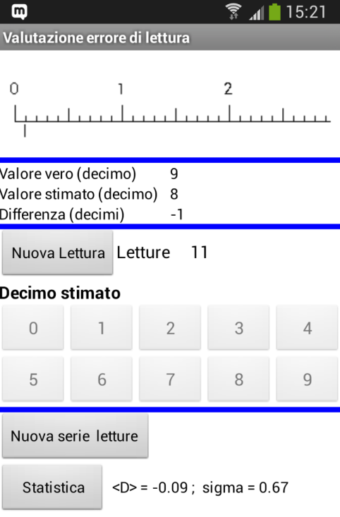
- Android app to check your ability
to interpolate between scale marks
- ErroriLettura.apk
(screenshot)
No dogmatism, please! - Other apps from Google app store:
- Vernier Caliper Simulator (try to read the tenths without using the vernier)
- Extra links and recomended readings on the subject:
- J. D. Mollon, A. J. Perkins, Errors of judgement at Greenwich in 1796, Nature 380, 101 - 102 (14 Mar 1996) (for the pdf see here, or local copy)
- Ole Rømer and his determination of the speed of light (interessante sito in italiano)
- Dava Sobel, Longitude.
- ErroriLettura.apk
(screenshot)
- The ultimate confidence intervals calculator
- Simple example with two Causes and two effects (AIDS test).
- P(A|B) vs P(B|A).
- What is 'statistics'? [→"Lies , dammn lies and statistics"]:
descriptive statistics, probability theory, inference. - "Lies, damned lies and... Physics".
- Criticism of p-values (and of frequentistic methods in general).
References, links, etc.
- GdA, Bayesian reasoning in high energy physics.
Principles and applications:
Yellow Report CERN 99-03
- Chapter 1;
- Sections 2.1-2.6;
- Sections 3.3-3.5 (we shall come back to the 'details').
- About the "HERA events":
- BR_HERA_events.pdf
(pp. 21-22 from Bayesian Reasoning)
- see old scanned slides
- my "anti-publication"
- BR_HERA_events.pdf
(pp. 21-22 from Bayesian Reasoning)
- GdA & G. Degrassi, Higgs mass indirect determination: arXiv:hep-ph/9902226
(for the moment, just give a look to probability distribution of the Higgs boson mass under different hypotheses/data, i.e. figs. 3 and 5) - Wiki/Misuse_of_p-values
- 2016 "ASA statements on p-values", The American Statistician, 70:2 (2016) 129-133
- GdA, Bayesian reasoning versus conventional statistics in High Energy Physics, arXiv:physics/9811046
- GdA, Probably a discovery: Bad mathematics means rough scientific communication,
arXiv:1112.3620v2
(with Appendix on the December 2011 '3-σ Higgs'). - GdA, The Waves and the Sigmas (To Say Nothing of the 750 GeV Mirage), arXiv:1609.01668
For the moment, just read sections 1-5. - Betting against the first 5-sigma discovery claim from LHC: footnote 31, p. 21 of https://arxiv.org/abs/1609.01668.
- Is Most Published Research Wrong?: YouTube by Veritasium (very well done!);
- I Fooled Millions Into Thinking Chocolate Helps Weight Loss. Here's How, John Bohannon, GIZMODO, 27 May 2015.
- GdA, From Observations to Hypotheses: Probabilistic Reasoning Versus Falsificationism and its Statistical Variations, arXiv:physics/0412148
- GdA, About the proof of the so called exact classical confidence intervals. Where is the trick?, https://arxiv.org/abs/physics/0605140
- More on model thinking applied to inference and prediction.
- Sources of uncertainty.
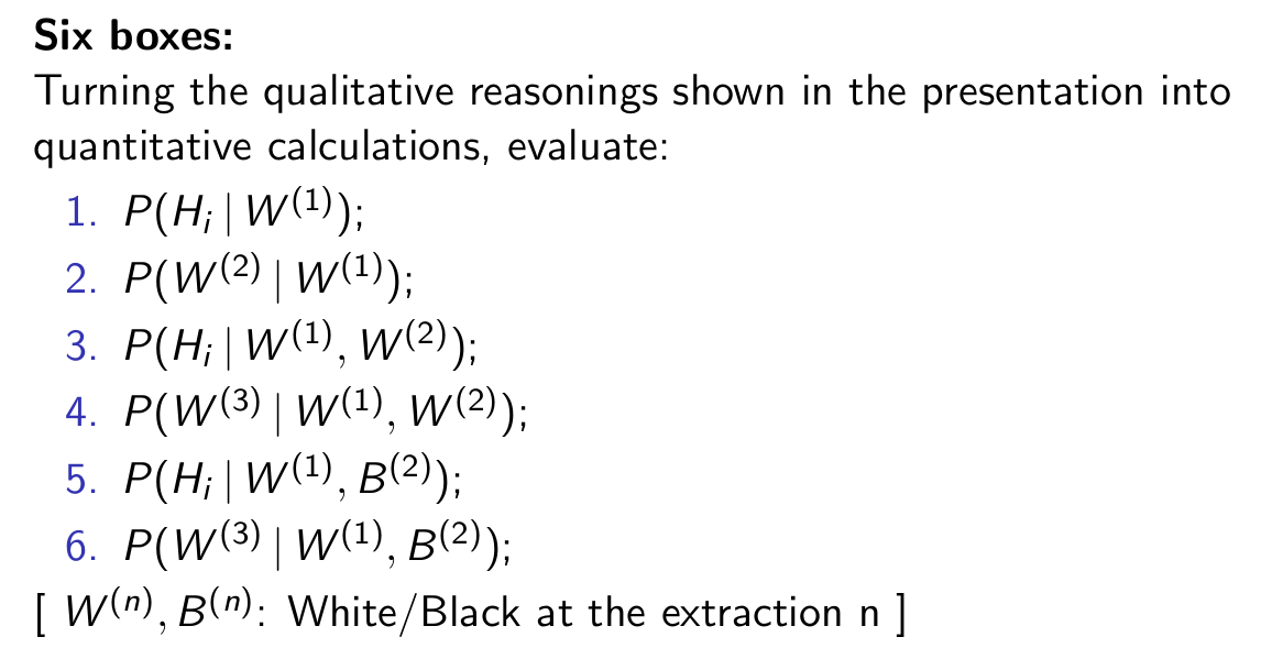
- The six box toy experiment.
- Dependence of probability from the state of information
(Monthy Hall problem and its variation). - Meaning of subjective probability (degree of belief).
- Beliefs and bets.
- On the standard text book 'definitions' of probability.
- Basic rules of probability, with remarks og the 4th rule (probability is always) conditioned.
- The Laplace's Bayes Theorem,
with home work:- AIDS problem;
- two rings (gold/silver) and three boxes;
- particle identification;
- Some questions concerning the six box toy experiment:
- Analyse the 'experiment' done during the questions, i.e. evaluate how all probabilities of interest evolve as the extractions proceed.
- Uncertain numbers — an introduction.
- More about the importance of the state of information in our scientific judgements (cows and sheep jokes).
- Extending the past to the future (possibly avoiding the end of the inductivist turkey...).
- Criticism to randomness (just metioned).
[And remember that we regularly use pseudorandom number generators!]
References, links, etc.
- GdA, Teaching statistics in the physics curriculum.
Unifying and clarifying role of subjective probability,
AJP 67, issue 12 (1999) 1260-1268; arXiv:physics/9908014 [limited to Sections II and IV, for the moment] - Plato and a platypus walk into a bar
- Conferenza di Alessandro Barbero, interessante non (sol)tanto per i fatti storici trattati, ma perché i metodi moderni degli storici ricordano quelli che abbiamo discusso, nelle prime lezioni, per fare scienza.
- More on the so called Bayes theorem
- Laplace's teaching and the original sinn of the frequentists.
- Bayes factors
- Bayesian networks and analysis of (a variation of) the six box toy experiment using Hugin.
- Uncertain numbers and probability functions.
- Summaries of probability distribution (do not confuse RMS with σ!)
- Introduction to Monte Carlo methods for generator (hit/miss and inversion of the cumulative distribution) and integration.
- Bernoulli process and related distributions (Geometric, Binomial and Pascal).
- Poisson process and related distributions (Poisson, Exponential and Erlang).
- Bernoulli theorem: meaning and misundestrandings.
References, links, etc.
- Veritasium on Bayes theorem
- GdA, The Gauss' Bayes Factor, arXiv:2003.10878 [math.HO]
- Hugin:
Hugin Lite (free → download)
- Tutorials.
- Examples provided by the company: Samples
- Ready-to-use models based on the six-boxes toy experiment:
- six_boxes.oobn (basic model)
- six_boxes_dado.oobn (+ 'reporter' who might err/lie)
- six_boxes_prep_dado.oobn (+ uncertainty on the box preparation) → model shown today.
- Try to edit the models (within HUGIN), changing the probability tables, adding nodes, etc..
- Try to write from scratch the (minimalist) model to solve
the AIDS problem, using the number suggested in the slides
for easy comparison.
just two nodes- Infected, with two possible states, Yes and No;
- Analysis result, with two possible states, Positive/ and Negative.
- Modify the previous model, using equiprobable
priors for Infected/Non-Infected:
- compare the result with the those obtained with (roughly) realistic priors;
- compare the result with the wrong one suggested in the first lecture.
- Think then to the possible practical utility of using equiprobable priors.
- Netica: a valid alternative to Hugin, thanks also to the many available whose interest goes beyond the specific package.
- A useful vademecum: Probability Distributions:
-
Lecture notes "Probabilità e incertezze di misura"
(in Italian, but you might recognize the formulae of the slides)
- Parte 1
- Chapter 4, pp. 61-80
(some details will be covered in the second part of the course);
- Chapter 5, till pp. 95
- Chapter 4, pp. 61-80
(some details will be covered in the second part of the course);
- Parte 2
- Chapters 6;
- Chapter 7 (till p. 175);
- Chapter 8 (only 8.12.1-8.12.4).
- Parte 3
- Sec. 10.9
- Parte 1
- Some R commands:
- barplot(table(outer(1:6, 1:6, '+'))/36) # sum of 2 dice
- barplot(table(outer(1:6, 1:6, '+'))/36, col='cyan', xlab='s', ylab='f(s)')
- barplot(table(factor( outer(1:6, 1:6), levels=1:36))) # product of 2 dice
- n=10; p=0.3; x=0:n; P=dbinom(x,n,p); barplot(P, names=x)
- n=100; dbinom(n,n,1/n)
- n=100; dbinom(n,n,1/n, log=TRUE)/log(10)
- More suggested homework
- Write a random number generator, using the hit/miss
method, in order to simulate a binomial distribution
with, e.g., n=10 and p=1/2
Obviously, one can use R and just issue the following command (with 1000 numbers), which includes graphics:
N=100; n=10; p=1/2; barplot(table(rbinom(N, 10, p))/N) ↠ compare the results. - Write an exponential random number generator
using the method of the inverse of the cumulative distribution.
Again, this would be the results obtained using directly R, for e.g. τ=5:
N=1000; tau=5; mean(rexp(N, 1/tau))
N=1000; tau=5; hist(rexp(N, 1/tau),nc=50, xlim=c(0,6*tau), prob=TRUE, col='cyan') - Entry test:
- Problem nr 7 (rather easy after today's lecture);
- Problem 6, not as trivial, but think/discuss about it.
- Write a random number generator, using the hit/miss
method, in order to simulate a binomial distribution
with, e.g., n=10 and p=1/2
- More on the so called Bayes theorem
- More on the six boxes
- Monte Carlo simulation of 100 extractions
- Comparison with frequentistic conclusions
- Markov and Cebicev disequalities
- More on Poisson processs
- decay lifetime vs half time of radioactive decays.
- Continuous probability distributions.
- Propation of uncertainties
- Central limit theorem and its importance
- Exact and MC propagation of uncertainties
- Criticism of `propagation prescriptions'
References, links, etc.
- GdA, More lessons from the six box toy experiment, https://arxiv.org/abs/1701.01143
- The very venerable proton...
- For the Fermi's Bayes theorem and the Gauss' Bayes factor, see here
- GdA, Bertrand 'paradox' reloaded,
https://arxiv.org/abs/1504.01361
→ besides the 'paradox', the paper contains details on exact tranformations of variables. - GdA, Asymmetric Uncertainties: Sources, Treatment and Potential Dangers, https://arxiv.org/abs/physics/0403086
- Lecture notes "Probabilità e incertezze di misura"
- Gauss' derivation of the Gaussian:
- Gauss, Theoria Motus Corporum Coelestium in Sectionibus Conicis Solem Ambientium, SECTIO TERTIA, pp. 205-224 (expecially p. 212).
- Gauss, Theory of the motion of the heavenly bodies moving about the sun in conic sections, Third Section, pp. 249-273 (expecially pp. 258-259).
- 'Gaussian trick' (→ Laplace approximation!)
- Asymmetric Uncertainties: Sources, Treatment and Potential Dangers, arXiv:physics/0403086.
- Some R commands/scripts:
- tau=5; n=10000; hist(-tau*log(runif(n)), nc=100, col='cyan')
- sum_square_wave.R (→ cartoon 'proof' of the CLT)
- sum_prod_2dice_CLT.R (→ other version, using the product of two dice as starting distribution)
- sum_z2.R (→ χ2)
- sum_z2_over_nu.R
- simple_gaussian_generator.R
- Pdf of the sum of two uniform distributions done with WolframAlpha
- Integrate[DiracDelta[s - x1 - x2], {x1, 0, 1}, {x2, 0, 1}];
- Click on "A Plain Text " and copy the result 'to Clipboard';
- Paste the result on the command window, adding the Plot instructions, that is
- In the simulated six box experiment we have observed
a white ball extracted about 25 times. But, because
technical reason you might have
making the calculations, let us assume
that this happened 23 times.
Assuming, as we new, that the choosen box was H1, i.e. the one containing 1 white and 4 black,- how would a particle physicist report such an extraordinary event in terms of 'sigmas'?
- So what?
- Homework on exact tranformations
- PDF of sum of two ('iid') asymmetric triangular distributions done analytically using Mathematica: [But it can be done more easily by MC, also extending it to many triangulars, using rtriang() included in the script triang.R available in the R web page]
- Logical vs `stocastic' (probabilistic) dependence
- Exercises on (rather elementary) exact propagation
(and `Monte Carlo checks') - Another way to perform exact propagations
- A 'curious' trasformation: Y(x)=FX(x)
- From exponential to Erlang and Gamma (and χ2)
- Multivariate distributions
- Bivariate normal distribution and its importance
(and extension to $n$ dimensions) - Gaussian Trick' in many dimensions (use and misuse)
References, links, etc.
- Todays' slides.
-
Lecture notes "Probabilità e incertezze di misura",
Parte 3
- Secs. 9.1-9.7 (some 'details' not shown during the lecture)
- Sec. 9.10-9.11 (9.12 left to self reading)
- GdA, Learning about probabilistic inference and
forecasting by playing with multivariate normal distributions
(with examples in R),
https://arxiv.org/abs/1504.02065, Secs. 1-3.
- Logical vs `stocastic' (probabilistic) dependence
- More on linear combinations of uncertain numbers
'Propagation' of covariance matrix - Linearization of non-linear functions
Special case of monomial forms - More on multivariate normal distributions
Conditioning on a set of variables - Extension of the box `experiment'
from n=6 to n → infinity
- Bayes' billiard and inference of Bernoulli's 'p
- Graphical models
- f(p) starting form a uniform prior: "Laplace' rule"
- meaning of E[p]
- "frequency based" evaluation of 'p'
- Special cases of x=0 and x=n
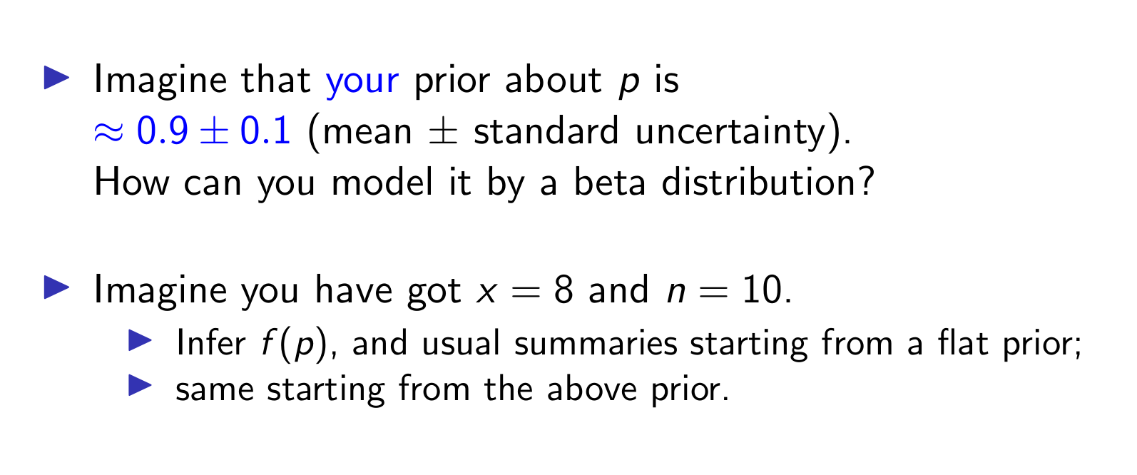
- Conjugate priors and Beta pdf
- Role of priors: be carefull! No dogmas or 'postulates'
- Predictive problem: qualitative/MC introduction
References, links, etc.
-
Lecture notes Probabilità e incertezze di misura,
Parte 2
- Secs. 8.14.1 (also 8.14.2-8.14.3, covering a previous lecture)
-
Lecture notes Probabilità e incertezze di misura,
Parte 3
- Secs. 10.1-10.3, 10.4.2, 10.5, 10.7-10.8, 10.13-10.14
-
Lecture notes Probabilità e incertezze di misura,
Parte 4
- Sec. 12.3
- GdA, CERN Yellow Report
on Bayesian reasoning in high energy physics.
Principles and applications,
Sec. 5.5.1 (Part 2) - GdA, https://arxiv.org/abs/2102.11022,
Sec. 4.1
(see also bottom table of Tab. 3, expecially to compare how the three farma companies have reported the "95% uncertainty interval", as mentioned during the lectures) - GdA, https://arxiv.org/abs/1504.02065, Sec. 9 → constraining the measured angles of a triangle.
- Getting familiar with the Beta pdf, e.g.
p<-seq(0,1,by=0.01); plot(p, dbeta(p, 3, 5), ty='l', col='blue', ylab='f(p)')
(Try also to use the suggested app) - Propagation of ... mistakes evaluating an efficiency
and its uncertainty:
rm23_07_propagation_of_mistakes.pdf - Problems suggested in the slides:
rm23_07_problems.pdf - Two other intersting problems: beta_problems.png
- More on the Bernoulli's p:
- case of x=0 and large n (e.g. very rare B.R.'s)
- Joint inference and prediction
- Inferring Poisson λ and process intensity r
(including special case of x=0, conjugate prior and predictive distribution) - Including background
- Inference and forecasting related to Gaussian distributions
- Practical introduction to JAGS (via rjags)
References, links, etc.
- Lecture notes Probabilità e incertezze di misura,
Parte 4
- Secs. 12.4
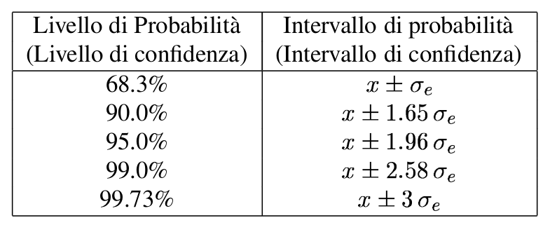
- Secs. 11.1-11.3, 11.6-11.7
(Note the table at pag. 315, in which I was using, at that time, 'confidence' and 'probability' as synonymous....) - Sec. 12.2 (in the light of the previous sections)
- GdA, CERN Yellow Report
on Bayesian reasoning in high energy physics.
Principles and applications (Part 2),
Sec. 5.4.1-5.4.3, 5.5.2. - GdA, https://arxiv.org/abs/1504.02065, Sec. 11: Propagation of evidence — some general remarks.
- An important case worth thinking a while (with R code):
- p=10^seq(-5,-1,len=100)
n1=100; plot(p, (1-p)^n1, ty='l', log='xy'); grid()
n2=1000; points(p, (1-p)^n2, ty='l', col='red')
- p=10^seq(-5,-1,len=100)
- Related important exercise:
- f(λ) for observed x=0;
- transform f(λ) into f(r), given the observation time T
- plot f(r) in log-log scale for different observation times T
- JAGS/rjags examples (see also dedicated web page)
- JAGS 'improperly' used as simple random generator:
- model file: simple_simulations.bug
- stearing script: simple_simulations.R
— simple_simulations_1.R
Moreovere, here is how to extract the individual histories and to make customized graphics:
simple_simulations_graphics.R
(run the script after the previous one, and cuctomize it at wish). - Inference and forecasting in the binomial case:
- inf_p_pred_jags.R
(model file included in the R script — convenient in the case of small models!)
- inf_p_pred_jags.R
- Inference and prediction from a Gaussian sample:
a feeling of what it is going on (and to customize the analysis/graphics at wish) - JAGS 'improperly' used as simple random generator:
- Use JAGS in order to solve
last lecture problem on the measurements
of the three internal angles of a triangle, conditioned on the value of their sum.
(And compare the results — including the correlation matrix! — with what is obtained from normal multivariate conditioning described in Sec. 9 of https://arxiv.org/abs/1504.02065) - Variation on the triangle problem: imagine that only α and β
are directly measured, while γ is deduced
from the the sum.
- How will the result change?
- In particular, compare the correlation matrices obtained in the two cases.
- introduction and asympotic results (n→∞);
- sufficient statistics;
- comments on 'standard' (even 'Bayesian'!) treatment of small samples (details left, for the moment, to self reading).
- Rejection sampling
- Importance sampling
- Markov Chain Monte Carlo
- A practical introduction by curious games
- Global and detailed balance conditions
- Metropolis algorithm
- Simulated annealing
- Gibbs sampler
- Applications to the 'binomial related problems'
- joint inference of p and x_fut
- yet another introduction to graphical models and the use of JAGS
- a self made Gibbs sampler
- solution by Metropolis
- solution by hit/miss (rejection sampling)
- numerical solution (proposed as exercise)
References, links, etc.
- For an introduction to MCMC, Metropolis and Gibbs sampler:
C. Andrieu et al., An introduction to MCMC for Machine Learning, Machine Learning, 50 (2003) 5-43,
https://doi.org/10.1023/A:1020281327116 - The Coursera mentioned during the lecture,
with main instructor Werner Krauth,
(re-)starts right today!
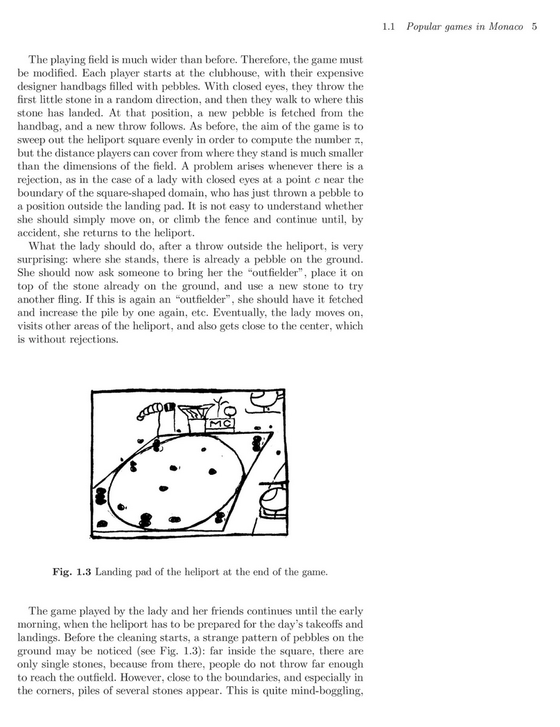
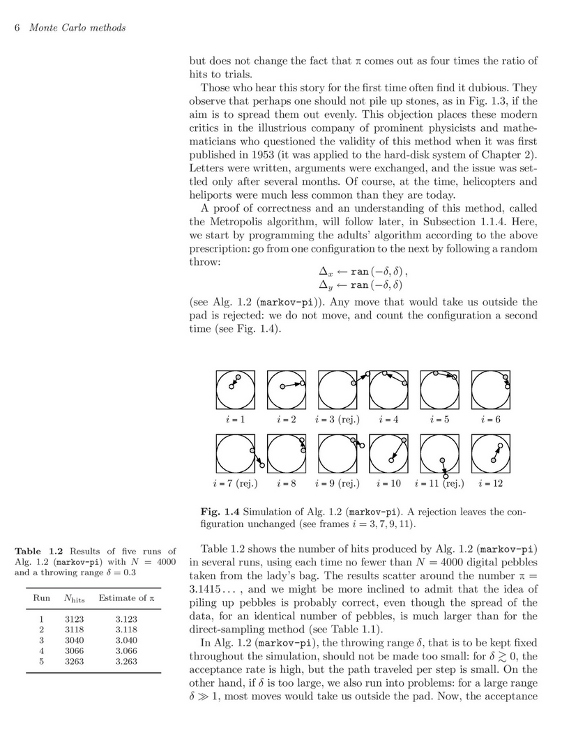
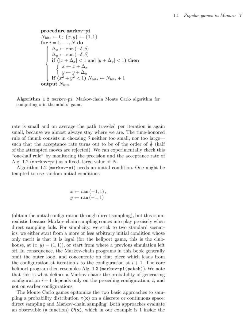
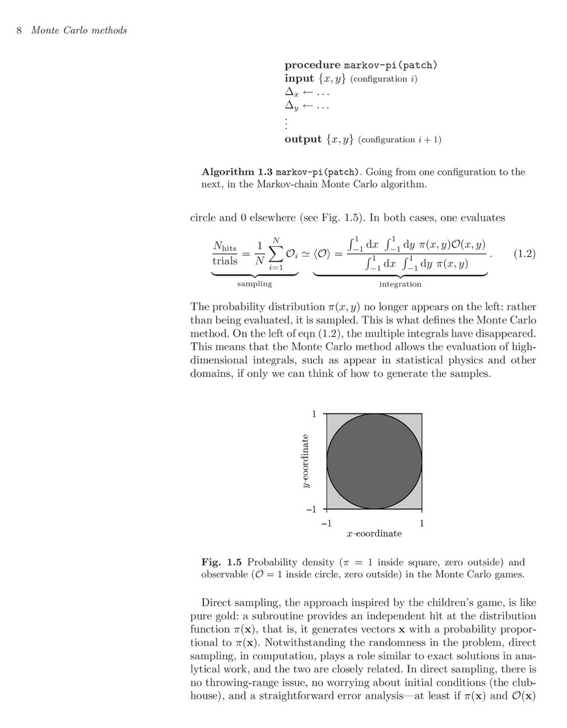
His book is Statistical Mechanics: Algorithms and Computations (same title of the Coursera)
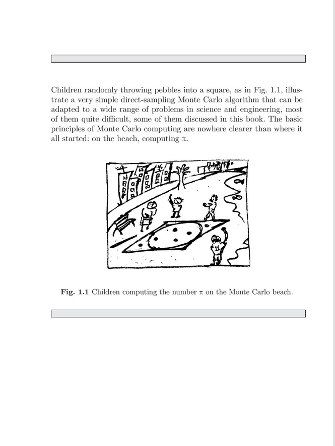
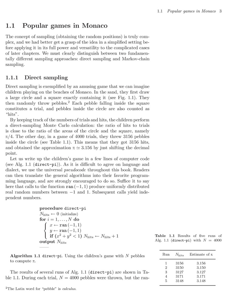
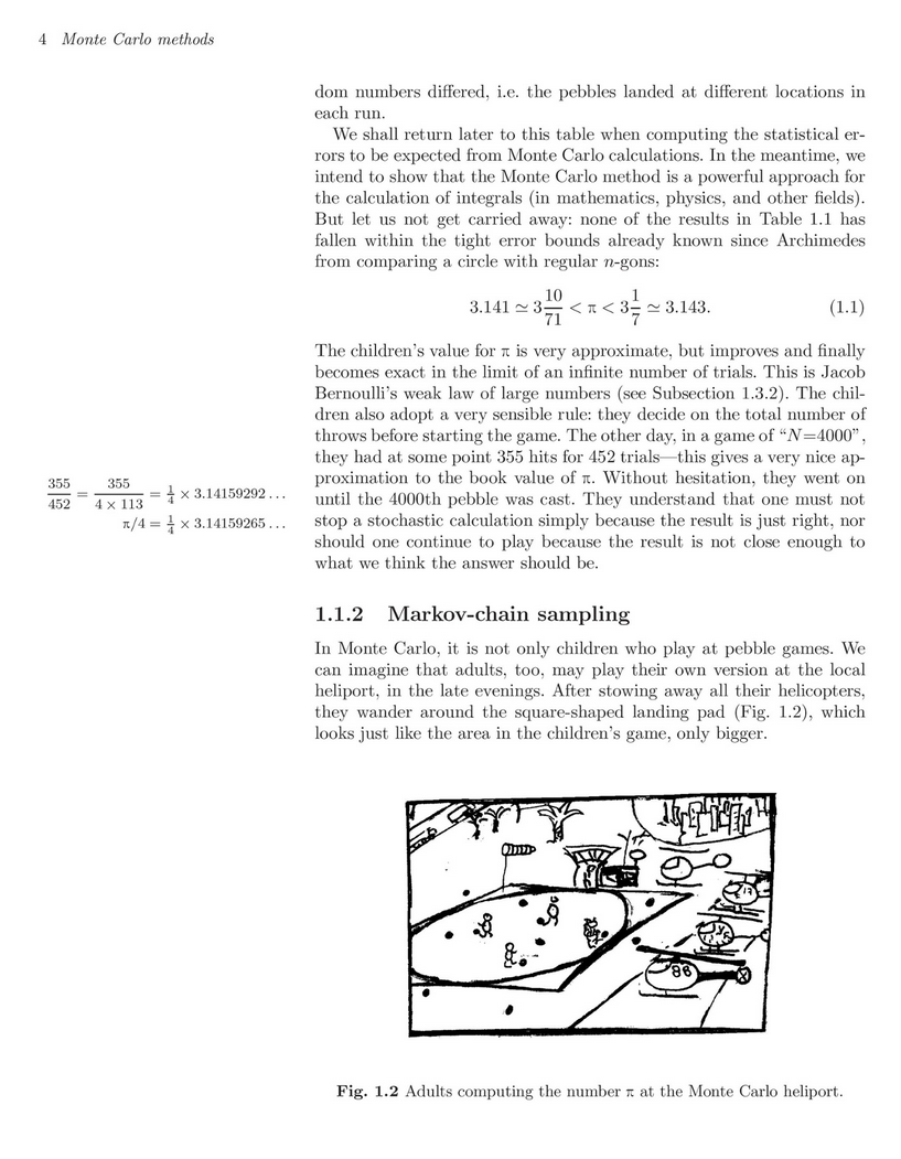
Good news: the examples of children and adults playing throwing stones are readible in the Amazon preview, pp. 1-9: - For Metropolis, Fermi & Co., see e.g. in this hystoric excursus and references therein.
- Lecture notes Probabilità e incertezze di misura,
Parte 4
- Sec. 11.6
- GdA, Jeffreys priors versus experienced physicist priors — arguments against objective Bayesian theory
- R scripts
- importance_sampling.R
- mcmc_unbound.R
- mcmc_square.R
- mcmc_3states.R
- update_mu.R
- T_to_t.R
- mcmc_3states_eigen.R
- first_metropolis.R
- metropolis.R
- metropolis_annealing.R
- gibbs_bivariate_normal.R
- gibbs_bivariate_normal_history.R
- inf_p_pred_gibbs.R
- inf_p_pred_metropolis.R
- inf_p_pred_hit-miss.R
- inf_p_pred_jags_1.R (same as inf_p_pred_jags.R of last lecture, but with the results provided in the same format as those of the other three methods)
- Gaussian (small) samples:
- standard (Bayesian) approch and criticism;
- application of MCMC via Gibbs sampling.
- More on the binomial/Poisson models
- Inferring binomial n given x and p
- A general graphical model for a counting experiment, including uncertain efficiency and background.
- Covid related applications:
- inferring the proportion of infected people in a population;
- vaccine efficacy.
- BAT (Bayesian Analisis Tool — just advertised)
References, links, etc.
- Slides of the lecture, posted in the usual place.
- Lecture notes Probabilità e incertezze di misura,
Parte 4
- Sec. 11.6 (containing also the case of a uniform prior in log σ not discussed during the lecture).
- GdA, Jeffreys priors versus experienced physicist priors — arguments against objective Bayesian theory
- Probabilistic issues concerning Covid:
→ mainly focus on the figures reproduced in the slides;
→ note the analogies with many issues of physics relevance, like measuring efficiencies, etc. - BAT
- BAT: The Bayesian Analysis Toolkit
- Use in the HEP community
- Getting started with BAT (and Root)
(Web page of end 2013, no guarantee that the procedures still work, but you can get an idea)
- Problems:
- It is highly recommended to try to solve the suggested problems.
- Continuation of the problem of inferring n
given p=0.75 and x=10:
- infer the Poisson λ which could have been the cause of n;
- then, infer the intensity of the Poisson process
r assuming a mesurement time of 100 days.
(report the result in s-1); - finally, evaluate how f(r) change if
we assume a precise value of
rB=10-6 s-1
for the rate of background
(repeat it also for rB=0.5x10⁻⁶ s-1 and rB=0.1x10⁻⁶ s-1).
- Some old and new problems, in particular
- exercizes on exact transformations;
- two envelops: hold or change?
- three prisoner problem.
- Coherent bet and basic rules of probability.
- p-values vs Bayes Factors (and much more!)
(based on the real case of 2015 GW's)
References, links, etc.
- Slides of the lecture, posted in the usual place.
- Lecture notes Probabilità e incertezze di misura, Parte 1, Sec. 4.2, 4.4-4.9.
- GdA, Bayesian reasoning in high energy physics. Principles and applications,
CERN Yellow Report 99-03, July 1999 (local copy),
Secs. 1.7-1.8, 2.1 (in particular the footnotes there); Ch. 3 up to Sec, 3.5; - GdA, The Waves and the Sigmas (To Say Nothing of the 750 GeV Mirage),
arXiv:1609.01668 [physics.data-an].
(More on the subject here). - GdA, Probability, Propensity and Probability of Propensities (and of Probabilities),
arXiv:1612.05292 [math.HO].
(More on the subject here and here.)
- Some old and new problems:
- exercizes on exact transformations;
- propagation of uncertainties on the A4 paper data
(for the propagation formulae see Slides of Lecture nr. 8, pp. 3-10).
- Uncertainties due to systematics
- General introduction
- Exact solution of the simple important of offset systematics
R scripts
References, links, etc.
- Slides of the lecture, posted in the usual place.
- GdA, Role and meaning of subjective probability:
some comments on common misconceptions,
arXiv:physics/0010064 [physics.data-an] - CERN Yellow Report 99-03
- Sec. 2.10.3 (local copy of Part 1)
- Sec. 5.6 (local copy of Part 2)
- Sec. 8.8 (local copy of Part 3)
- Some old and new problems:
- reprocuctive property of Erlang, Gamma and $\chi^2$.
- Example of the use of the technique of complementing the exponential
- Uncertainties due to systematics
- Reminder of 'approach nr. 3';
- Application to offset and scale systematics.
- Fits (just parametric inference!):
- the importance of the underlying model;
- linear model: general approach; simplified
model (under well understood conditions) and
'least square' approximation (no 'principle'!) - case of uncertain σ;
- forecasting a future 'y' at a given xf.
R scripts
- linear_fit.R(*) (points regenerated at each run)
- linear_fit_data.R (simulated data used for the slides)
 (*)
Notes:
(*)
Notes:
- a small typo in the last line of the script has been corrected;
- modify the script in order to:
- evaluate and plot also μy(xf)
-
modify further the script in order to:
- consider two extrapolations, one at xf1=30
and the other at xf2=32:
→ make the two plots, evaluate expected values and variances;
→ draw the scatter plot and evaluate the correlation coefficient of yf(xf2) vs yf(xf1).
- consider two extrapolations, one at xf1=30
and the other at xf2=32:
References, links, etc.
- Slides of the lecture, posted in the usual place.
- GdA, Fits, and especially linear fits, with errors on both axes, extra variance of the data points and other complications, arXiv:physics/0511182 [physics.data-an]
- GdA, Fits (pdf version: Capitolo 12)
- CERN Yellow Report 99-03
- Sec. 6.1.1 (local copy of Part 2);
- pp. 106-107
- GdA, Le basi del metodo sperimentale: Fits (pdf version: Capitolo 12)

- Summaries on fits.
- 'Complications':
- arXiv:physics/0511182 [physics.data-an]
- For the backgroung that gave rise to the paper: \url{https://arxiv.org/abs/astro-ph/0606526}
- From general, probabilistic treatment to 'linear models'
solved bt Least Squares
(with worries about assumptions, simplification, etc.)
→ see details on the slides
→ R script applying the method on a polinomian fit: poly_fit.R - Model comparison: a very general introduction
References:- D.J.C. MacKay, Chapter 28} of
Information Theory, Inference, and Learning Algorithms
(a great book, freely available here) - I. Murray and Z. Ghahramani, A note on the evidence and Bayesian Occam’s razor
- C.E. Rasmussen and Z. Ghahramani, Occam's razor
- P. Astone, GdA and S. D'Antonio, Bayesian model comparison applied to the Explorer-Nautilus 2001 coincidence data, arXiv:gr-qc/0304096
- D.J.C. MacKay, Chapter 28} of
Information Theory, Inference, and Learning Algorithms
- On the possible deleterios effects of the covariance
matrics when used in fits:
On the use of the covariance matrix to fit correlated data
Related paper focusing a physics result, after the technical issues were solved: - Prior free upper/lower limits resulting for Frontier Physics searches:
- Inferring the intensity of Poisson processes at the limit of the detector sensitivity (with a case study on gravitational wave burst search)
- Constraints on the Higgs Boson Mass from Direct Searches and Precision Measurements
- Confidence limits: what is the problem? Is there the solution?
- Some R code:
→ Bozza-Taroni-Biederman, Bayes Factors for Forensic Decision Analyses with R (freely downloadable)
More on priors:- Jeffreys priors versus experienced physicist priors — arguments against objective Bayesian theory;
- Overcoming priors anxiety
(mentioned at the end of the lecture):- the die which gave an average of 4.5:
E.T. Jaynes, Where do we Stand on Maximum Entropy? (local copy) - the Bertrand 'paradox':
E.T. Jaynes, The Well-Posed Problem (local copy)
→ see Bertrand 'paradox' reloaded (with several technical issues of intersrest for this course, besides the 'paradox' itself).
- Unfolding:
- A Multidimensional unfolding method based on Bayes' theorem
→ more datails and code here. - Improved iterative Bayesian unfolding
→ more datails and code here.
- A Multidimensional unfolding method based on Bayes' theorem